Lesson 3: Introduction to Simple Linear Regression (SLR)

Nicky Wakim

2026-01-12

Learning Objectives

1. Identify the aims of your research and see how they align with the intended purpose of simple linear regression

2. Identify the simple linear regression model and define statistics language for key notation

3. Illustrate how ordinary least squares (OLS) finds the best model parameter estimates

4. Solve the optimal coefficient estimates for simple linear regression using OLS

5. Apply OLS in R for simple linear regression of real data

Process of regression data analysis

Model Selection

• Building a model

• Selecting variables

• Prediction vs interpretation

• Comparing potential models

Model Fitting

• Find best fit line

• Using OLS in this class

• Parameter estimation

• Categorical covariates

• Interactions

Model Evaluation

• Evaluation of model fit
• Testing model assumptions
• Residuals
• Transformations
• Influential points
• Multicollinearity

Model Use (Inference)

• Inference for coefficients
• Hypothesis testing for coefficients

• Inference for expected \(Y\) given \(X\)
• Prediction of new \(Y\) given \(X\)

Let’s start with an example

 

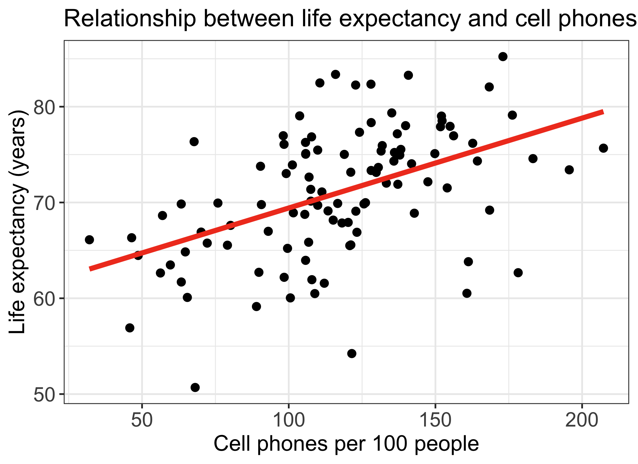
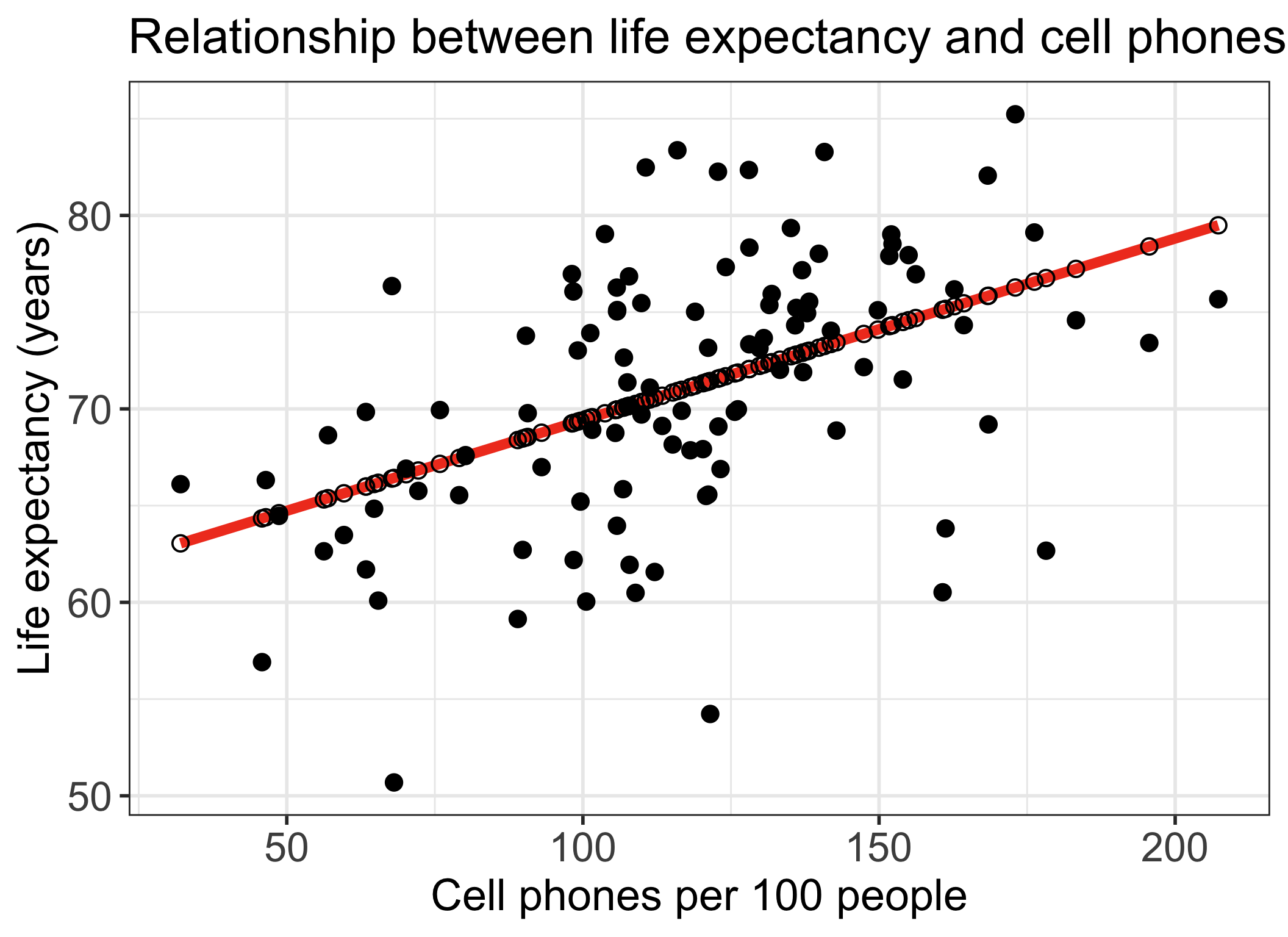
Life expectancy vs. cell phones

 

• Each point on the plot is for a different country/territory

 

• \(X\) = country’s number of cell phones per 100 people

 

• \(Y\) = country’s life expectancy (years)

\[\widehat{\text{life expectancy}} = 60.04 + 0.094\cdot\text{cell phones}\]

Reference: How did I code that?

gapm %>%
  ggplot(aes(x = cell_phones_100,
             y = life_exp)) +
  geom_point(size = 4) +
  geom_smooth(method = "lm", se = FALSE, size = 3, colour="#F14124") +
  labs(x = "Cell phones per 100 people",
       y = "Life expectancy (years)",
       title = "Relationship between life expectancy and cell phones") +
    theme(axis.title = element_text(size = 27), 
        axis.text = element_text(size = 25), 
        title = element_text(size = 25))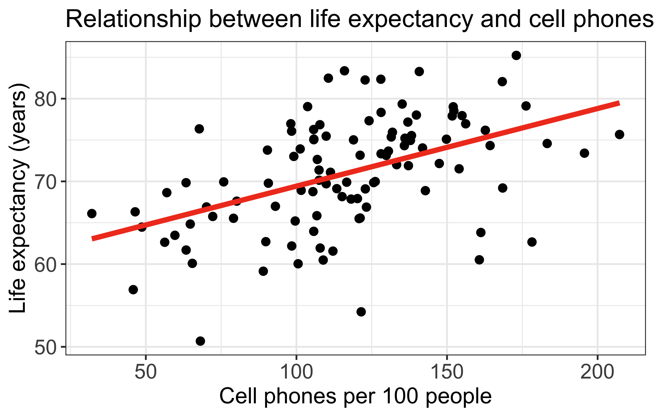

Research and dataset description

Research question: Is there an association between life expectancy and number of cell phones?

• Data file: gapminder.Rdata

• You can access my codebook here

• Data were downloaded from Gapminder

  • 2022 is the most recent year with the most complete data
  • Observational study measuring different characteristics of countries/territories, including population, health, environment, work, etc.

• Life expectancy = the average number of years a newborn child would live if current mortality patterns were to stay the same.

• Cell phones per 100 people is the number of cell phone subscriptions per 100 people in a given population, indicating the level of mobile phone use and accessibility.

 

Poll Everywhere Question 1

Get to know the data (1/3)

• Load data

load(here("data", "gapminder2022.RData"))

Get to know the data (2/3)

• Glimpse of the data

glimpse(gapm)

Rows: 105
Columns: 11
$ geo                 <chr> "afg", "alb", "are", "arg", "arm", "aze", "ben", "…
$ territory           <chr> "Afghanistan", "Albania", "UAE", "Argentina", "Arm…
$ life_exp            <dbl> 62.64, 76.07, 73.41, 75.37, 73.66, 71.37, 63.96, 7…
$ freedom_status      <chr> "NF", "PF", "NF", "F", "PF", "NF", "PF", "PF", "F"…
$ vax_rate            <dbl> 69, 99, 98, 94, 98, 96, 89, 99, 96, 96, 76, 88, 98…
$ co2_emissions       <dbl> 211455404, 294574910, 5324389134, 8574249437, 4512…
$ basic_sani          <dbl> 70.39219, 99.30948, 98.97272, 98.46960, 100.00000,…
$ happiness_score     <dbl> 12.81, 52.12, 67.38, 62.61, 53.82, 45.76, 42.17, 3…
$ income_level_4      <chr> "Low income", "Upper middle income", "High income"…
$ cell_phones_100     <dbl> 56.2655, 98.3950, 195.6250, 131.4840, 130.5400, 10…
$ basic_sani_80_above <chr> "Low access", "High access", "High access", "High …

Get to know the data (3/3)

• Get a sense of the summary statistics

gapm %>% 
  select(cell_phones_100,
         life_exp) %>% 
  summary()

 cell_phones_100     life_exp    
 Min.   : 32.06   Min.   :50.69  
 1st Qu.: 99.13   1st Qu.:66.11  
 Median :116.68   Median :71.52  
 Mean   :116.52   Mean   :70.97  
 3rd Qu.:137.18   3rd Qu.:75.67  
 Max.   :207.28   Max.   :85.23  

• Plot the individual variables

cell_phone_hist = gapm %>%
  ggplot(aes(x = cell_phones_100)) +
  geom_histogram() +
  labs(x = "Cell phones per 100 people",
       y = "Number of territories",
       title = "Distribution of cell phones per 100 people") +
    theme(axis.title = element_text(size = 20), 
        axis.text = element_text(size = 18), 
        title = element_text(size = 20))

life_exp_hist = gapm %>%
  ggplot(aes(x = life_exp)) +
  geom_histogram() +
  labs(x = "Life expectancy (years)",
       y = "Number of territories",
       title = "Distribution of life expectancy") +
    theme(axis.title = element_text(size = 20), 
        axis.text = element_text(size = 18), 
        title = element_text(size = 20))

grid.arrange(cell_phone_hist, life_exp_hist, nrow=2)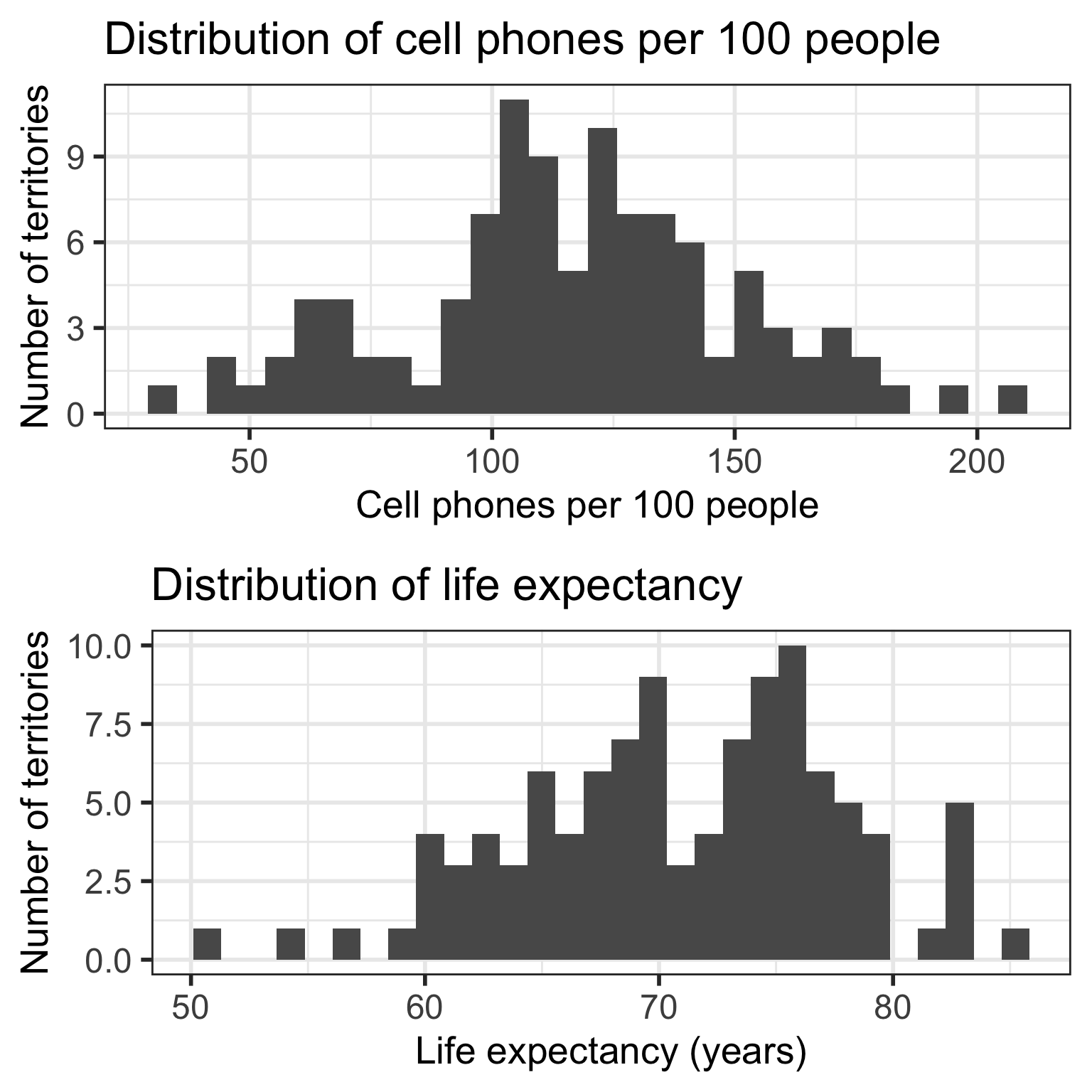

Poll Everywhere Question 2

Learning Objectives

1. Identify the aims of your research and see how they align with the intended purpose of simple linear regression

2. Identify the simple linear regression model and define statistics language for key notation

3. Illustrate how ordinary least squares (OLS) finds the best model parameter estimates

4. Solve the optimal coefficient estimates for simple linear regression using OLS

5. Apply OLS in R for simple linear regression of real data

Questions we can ask with a simple linear regression model

• How do we…
  • calculate slope & intercept?
  • interpret slope & intercept?
  • do inference for slope & intercept?
    • CI, p-value
  • do prediction with regression line?
    • CI for prediction?
• Does the model fit the data well?
  • Should we be using a line to model the data?
• Should we add additional variables to the model?
  • multiple/multivariable regression

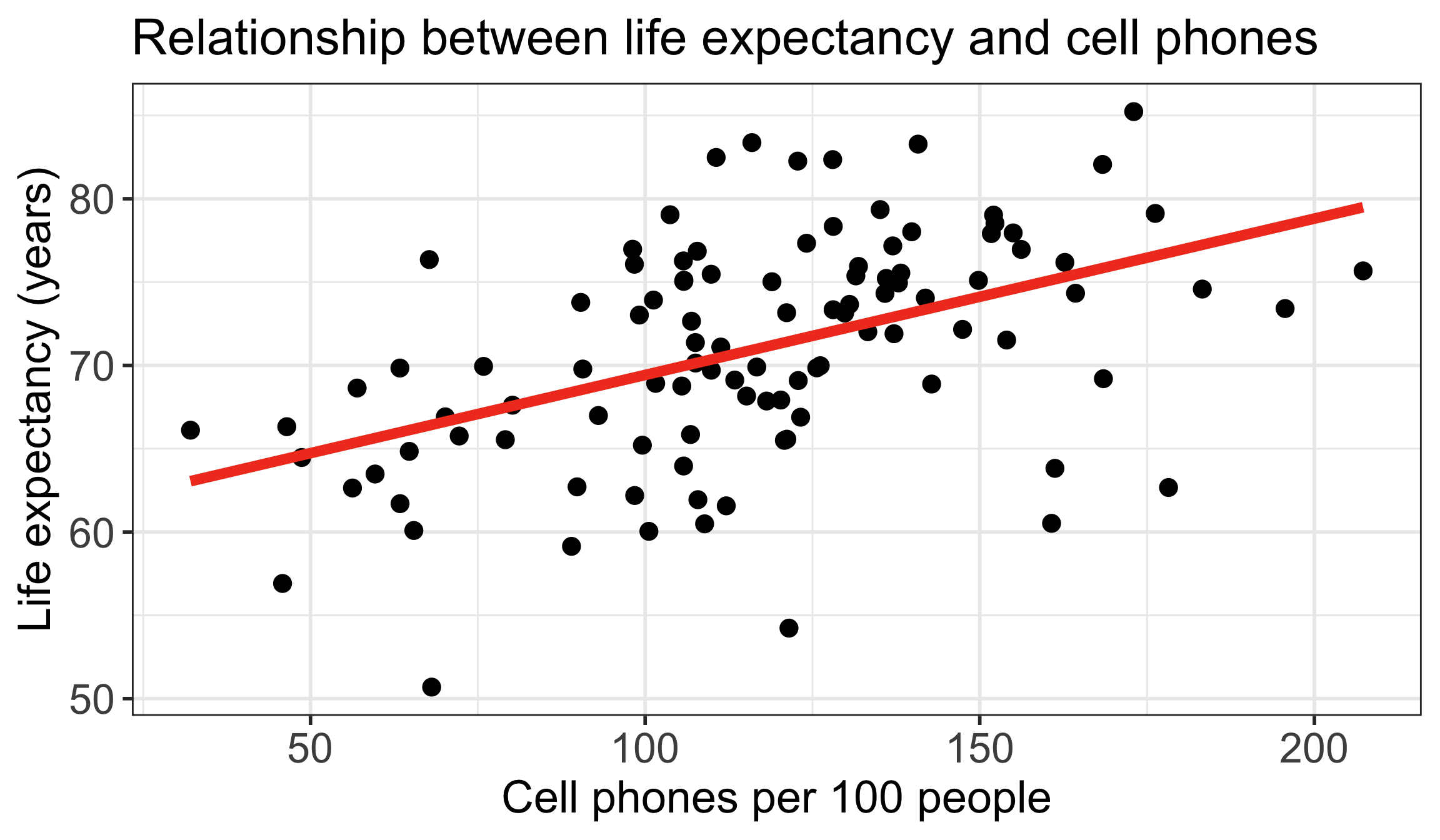
\[\widehat{\text{life expectancy}} = 60.04 + 0.094\cdot\text{cell phones}\]

Association vs. prediction

Association

• What is the association between countries’ life expectancy and cell phones?
• Use the slope of the line or correlation coefficient

Prediction

• What is the expected life expectancy for a country with a specified number of cell phones per 100 people?    

\[\widehat{\text{life expectancy}} = 60.04 + 0.094\cdot\text{cell phones}\]

Three types of study design (there are more)

Experiment

• Observational units are randomly assigned to important predictor levels

  • Random assignment controls for confounding variables (age, gender, race, etc.)

  • “gold standard” for determining causality

  • Observational unit is often at the participant-level

Quasi-experiment

• Participants are assigned to intervention levels without randomization

• Not common study design

Observational

• No randomization or assignment of intervention conditions

• In general cannot infer causality

  • However, there are casual inference methods…

Let’s revisit the regression analysis process

Model Selection

• Building a model

• Selecting variables

• Prediction vs interpretation

• Comparing potential models

Model Fitting

• Find best fit line

• Using OLS in this class

• Parameter estimation

• Categorical covariates

• Interactions

Model Evaluation

• Evaluation of model fit
• Testing model assumptions
• Residuals
• Transformations
• Influential points
• Multicollinearity

Model Use (Inference)

• Inference for coefficients
• Hypothesis testing for coefficients

• Inference for expected \(Y\) given \(X\)
• Prediction of new \(Y\) given \(X\)

Poll Everywhere Question 3

Learning Objectives

1. Identify the aims of your research and see how they align with the intended purpose of simple linear regression

2. Identify the simple linear regression model and define statistics language for key notation

3. Illustrate how ordinary least squares (OLS) finds the best model parameter estimates

4. Solve the optimal coefficient estimates for simple linear regression using OLS

5. Apply OLS in R for simple linear regression of real data

Simple Linear Regression Model

The (population) regression model is denoted by:

 

\[Y = \beta_0 + \beta_1X + \epsilon\]

 

Observable sample data

• \(Y\) is our dependent variable

  • Aka outcome or response variable

• \(X\) is our independent variable

  • Aka predictor, regressor, exposure variable

Unobservable population parameters

• \(\beta_0\) and \(\beta_1\) are unknown population parameters

• \(\epsilon\) (epsilon) is the error about the line

  • It is assumed to be a random variable with a…

    • Normal distribution with mean 0 and constant variance \(\sigma^2\)

    • i.e. \(\epsilon \sim N(0, \sigma^2)\)

Simple Linear Regression Model (another way to view components)

The (population) regression model is denoted by:

 

\[Y = \beta_0 + \beta_1X + \epsilon\]

 

Components

\(Y\)	response, outcome, dependent variable
\(\beta_0\)	intercept
\(\beta_1\)	slope
\(X\)	predictor, covariate, independent variable
\(\epsilon\)	residuals, error term

If the population parameters are unobservable, how did we get the line for life expectancy?

 

Note: the population model is the true, underlying model that we are trying to estimate using our sample data

• Our goal in simple linear regression is to estimate \(\beta_0\) and \(\beta_1\)

Poll Everywhere Question 4

Regression line = best-fit line

\[\widehat{Y} = \widehat{\beta}_0 + \widehat{\beta}_1 X \]

• \(\widehat{Y}\) is the predicted outcome for a specific value of \(X\)
• \(\widehat{\beta}_0\) is the intercept of the best-fit line
• \(\widehat{\beta}_1\) is the slope of the best-fit line, i.e., the increase in \(\widehat{Y}\) for every increase of one (unit increase) in \(X\)
  • slope = rise over run

Simple Linear Regression Model

Population regression model

Think of this as proposed model before we fit the data

\[Y = \beta_0 + \beta_1X + \epsilon\]

 

Components

\(Y\)	response, outcome, dependent variable
\(\beta_0\)	intercept
\(\beta_1\)	slope
\(X\)	predictor, covariate, independent variable
\(\epsilon\)	residuals, error term

Estimated regression line

Think of this as the actualized model after we fit data

\[\widehat{Y} = \widehat{\beta}_0 + \widehat{\beta}_1X\]

 

Components

\(\widehat{Y}\)	estimated expected response given predictor \(X\)
\(\widehat{\beta}_0\)	estimated intercept
\(\widehat{\beta}_1\)	estimated slope
\(X\)	predictor, covariate, independent variable

We get it, Nicky! How do we estimate the regression line?

First let’s take a break!!

Learning Objectives

1. Identify the aims of your research and see how they align with the intended purpose of simple linear regression

2. Identify the simple linear regression model and define statistics language for key notation

3. Illustrate how ordinary least squares (OLS) finds the best model parameter estimates

4. Solve the optimal coefficient estimates for simple linear regression using OLS

5. Apply OLS in R for simple linear regression of real data

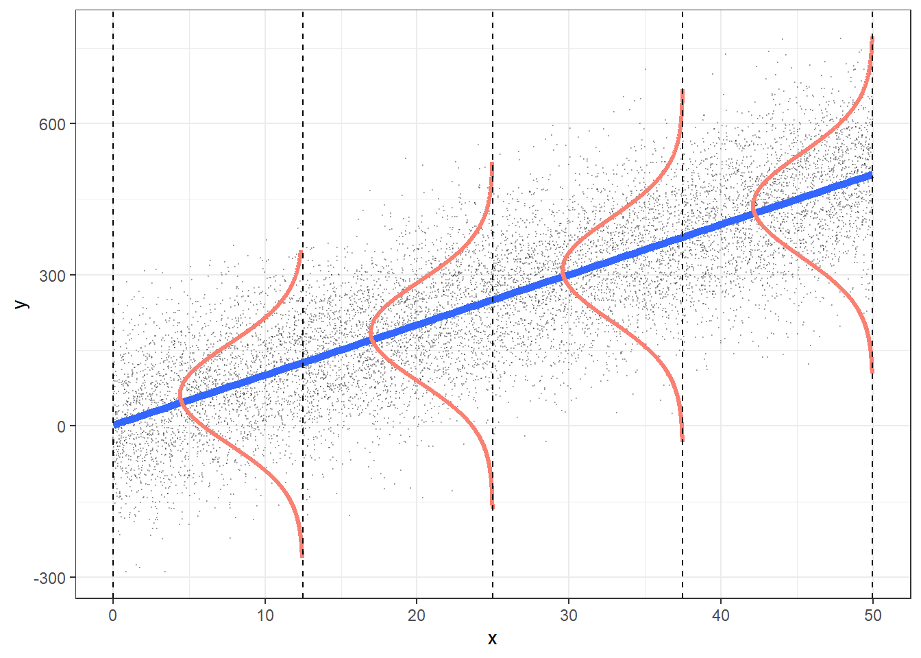
It all starts with a residual…

• Recall, one characteristic of our population model was that the residuals, \(\epsilon\), were Normally distributed: \(\epsilon \sim N(0, \sigma^2)\)

• In our population regression model, we had: \[Y = \beta_0 + \beta_1X + \epsilon\]

• We can also take the average (expected) value of the population model

• We take the expected value of both sides and get:

\[\begin{aligned} E[Y] & = E[\beta_0 + \beta_1X + \epsilon] \\ E[Y] & = E[\beta_0] + E[\beta_1X] + E[\epsilon] \\ E[Y] & = \beta_0 + \beta_1X + E[\epsilon] \\ E[Y|X] & = \beta_0 + \beta_1X \\ \end{aligned}\]

• We call \(E[Y|X]\) the expected value (or average) of \(Y\) given \(X\)

So now we have two representations of our population model

With observed \(Y\) values and residuals:

\[Y = \beta_0 + \beta_1X + \epsilon\]

With the population expected value of \(Y\) given \(X\):

\[E[Y|X] = \beta_0 + \beta_1X\]

Using the two forms of the model, we can figure out a formula for our residuals:

\[\begin{aligned} Y & = (\beta_0 + \beta_1X) + \epsilon \\ Y & = E[Y|X] + \epsilon \\ Y - E[Y|X] & = \epsilon \\ \epsilon & = Y - E[Y|X] \end{aligned}\]

And so we have our true, population model, residuals!

This is an important fact! For the population model, the residuals: \(\epsilon = Y - E[Y|X]\)

Back to our estimated model

We have the same two representations of our estimated/fitted model:

With observed values:

\[Y = \widehat{\beta}_0 + \widehat{\beta}_1X + \widehat{\epsilon}\]

With the estimated expected value of \(Y\) given \(X\):

\[\begin{aligned} \widehat{E}[Y|X] & = \widehat{\beta}_0 + \widehat{\beta}_1X \\ \widehat{E[Y|X]} & = \widehat{\beta}_0 + \widehat{\beta}_1X \\ \widehat{Y} & = \widehat{\beta}_0 + \widehat{\beta}_1X \\ \end{aligned}\]

Using the two forms of the model, we can figure out a formula for our estimated residuals:

\[\begin{aligned} Y & = (\widehat{\beta}_0 + \widehat{\beta}_1X) + \widehat\epsilon \\ Y & = \widehat{Y} + \widehat\epsilon \\ \widehat\epsilon & = Y - \widehat{Y} \end{aligned}\]

This is an important fact! For the estimated/fitted model, the residuals: \(\widehat\epsilon = Y - \widehat{Y}\)

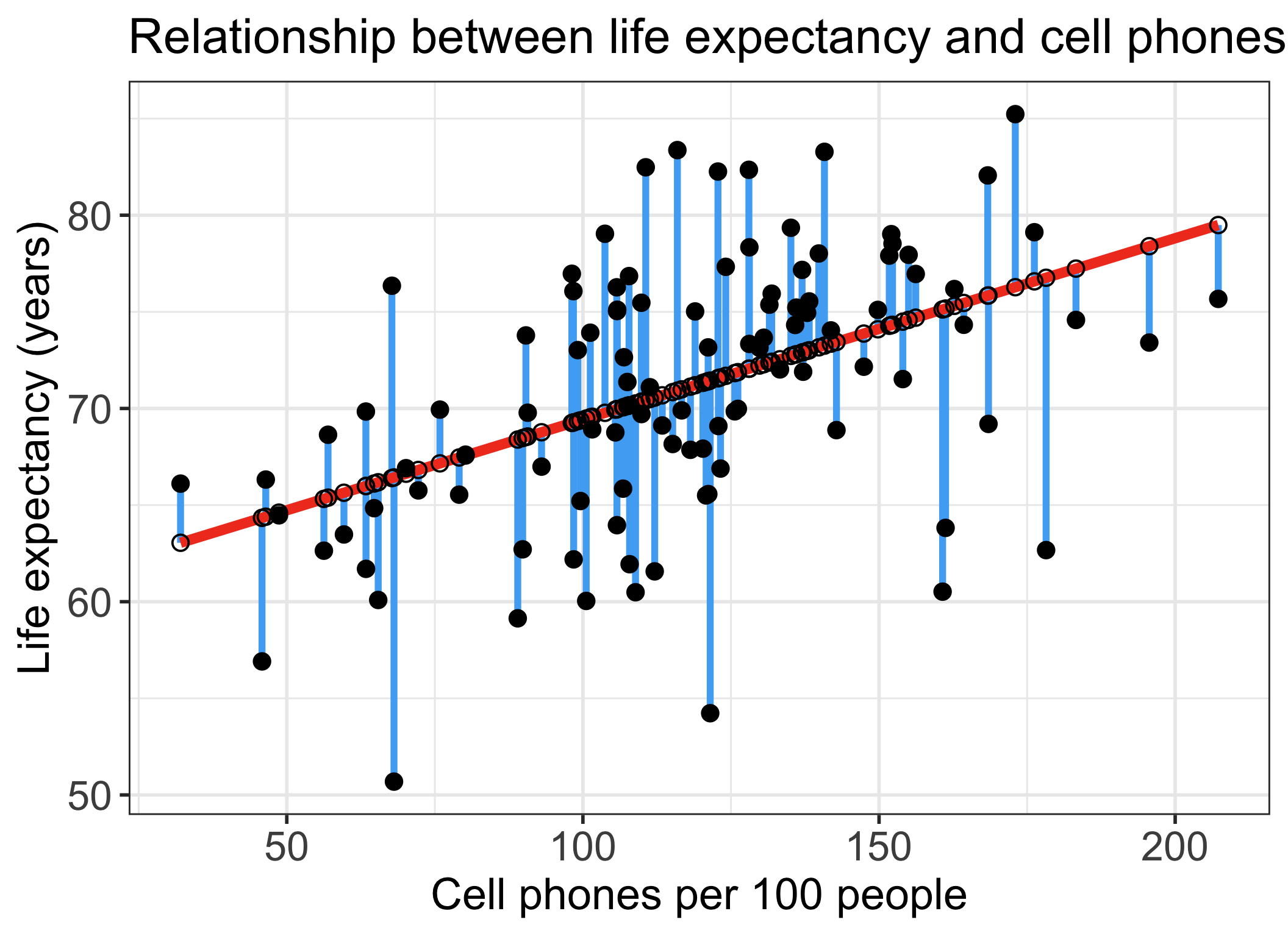
Residuals for observation \(i\) in the estimated/fitted model

• Observed values for each country \(i\): \(Y_i\)
  • Value in the dataset for country \(i\)
• Fitted value for each country \(i\): \(\widehat{Y}_i\)
  • Value that falls on the best-fit line for a specific \(X_i\)
  • If two individuals have the same \(X_i\), then they have the same \(\widehat{Y}_i\)

Residuals for observation \(i\) in the estimated/fitted model

• Observed values for each individual \(i\): \(Y_i\)

  • Value in the dataset for individual \(i\)

• Fitted value for each individual \(i\): \(\widehat{Y}_i\)

  • Value that falls on the best-fit line for a specific \(X_i\)
  • If two individuals have the same \(X_i\), then they have the same \(\widehat{Y}_i\)

• Residual for each individual: \(\widehat\epsilon_i = Y_i - \widehat{Y}_i\)

  • Difference between the observed and fitted value

Poll Everywhere Question 5

So what do we do with the residuals?

• We want to minimize the residuals

  • Aka minimize the difference between the observed \(Y\) value and the estimated expected response given the predictor ( \(\widehat{E}[Y|X]\) )

• We can use ordinary least squares (OLS) to do this in linear regression!

• Idea behind this: reduce the total error between the fitted line and the observed point (error between is called residuals)

  • Vague use of total error: more precisely, we want to reduce the sum of squared errors
  • We need to mathematically define this!

 

 

• Note: there are other ways to estimate the best-fit line!!

  • Example: Maximum likelihood estimation

Learning Objectives

1. Identify the aims of your research and see how they align with the intended purpose of simple linear regression

2. Identify the simple linear regression model and define statistics language for key notation

3. Illustrate how ordinary least squares (OLS) finds the best model parameter estimates

4. Solve the optimal coefficient estimates for simple linear regression using OLS

5. Apply OLS in R for simple linear regression of real data

Setting up for ordinary least squares

• Sum of Squared Errors (SSE)

\[ \begin{aligned} SSE & = \displaystyle\sum^n_{i=1} \widehat\epsilon_i^2 \\ SSE & = \displaystyle\sum^n_{i=1} (Y_i - \widehat{Y}_i)^2 \\ SSE & = \displaystyle\sum^n_{i=1} (Y_i - (\widehat{\beta}_0+\widehat{\beta}_1X_i))^2 \\ SSE & = \displaystyle\sum^n_{i=1} (Y_i - \widehat{\beta}_0-\widehat{\beta}_1X_i)^2 \end{aligned}\]

Things to use

• \(\widehat\epsilon_i = Y_i - \widehat{Y}_i\)

• \(\widehat{Y}_i = \widehat\beta_0 + \widehat\beta_1X_i\)

Then we want to find the estimated coefficient values that minimize the SSE!

Steps to estimate coefficients using OLS

1. Set up SSE (previous slide)

2. Minimize SSE with respect to coefficient estimates

   • Need to solve a system of equations

3. Compute derivative of SSE wrt \(\widehat\beta_0\)

4. Set derivative of SSE wrt \(\widehat\beta_0 = 0\)

5. Compute derivative of SSE wrt \(\widehat\beta_1\)

6. Set derivative of SSE wrt \(\widehat\beta_1 = 0\)

7. Substitute \(\widehat\beta_1\) back into \(\widehat\beta_0\)

2. Minimize SSE with respect to coefficients

• Want to minimize with respect to (wrt) the potential coefficient estimates ( \(\widehat\beta_0\) and \(\widehat\beta_1\))

• Take derivative of SSE wrt \(\widehat\beta_0\) and \(\widehat\beta_1\) and set equal to zero to find minimum SSE

\[ \dfrac{\partial SSE}{\partial \widehat\beta_0} = 0 \text{ and } \dfrac{\partial SSE}{\partial \widehat\beta_1} = 0 \]

• Solve the above system of equations in steps 3-6

3. Compute derivative of SSE wrt \(\widehat\beta_0\)

\[ SSE = \displaystyle\sum^n_{i=1} (Y_i - \widehat{\beta}_0-\widehat{\beta}_1X_i)^2 \]

\[\begin{aligned} \frac{\partial SSE}{\partial{\widehat{\beta}}_0}& =\frac{\partial\sum_{i=1}^{n}\left(Y_i-{\widehat{\beta}}_0-{\widehat{\beta}}_1X_i\right)^2}{\partial{\widehat{\beta}}_0}= \sum_{i=1}^{n}\frac{{\partial\left(Y_i-{\widehat{\beta}}_0-{\widehat{\beta}}_1X_i\right)}^2}{\partial{\widehat{\beta}}_0} \\ & =\sum_{i=1}^{n}{2\left(Y_i-{\widehat{\beta}}_0-{\widehat{\beta}}_1X_i\right)\left(-1\right)}=\sum_{i=1}^{n}{-2\left(Y_i-{\widehat{\beta}}_0-{\widehat{\beta}}_1X_i\right)} \\ \frac{\partial SSE}{\partial{\widehat{\beta}}_0} & = -2\sum_{i=1}^{n}\left(Y_i-{\widehat{\beta}}_0-{\widehat{\beta}}_1X_i\right) \end{aligned}\]

Things to use

• Derivative rule: derivative of sum is sum of derivative

• Derivative rule: chain rule

4. Set derivative of SSE wrt \(\widehat\beta_0 = 0\)

\[\begin{aligned} \frac{\partial SSE}{\partial{\widehat{\beta}}_0} & =0 \\ -2\sum_{i=1}^{n}\left(Y_i-{\widehat{\beta}}_0-{\widehat{\beta}}_1X_i\right) & =0 \\ \sum_{i=1}^{n}\left(Y_i-{\widehat{\beta}}_0-{\widehat{\beta}}_1X_i\right) & =0 \\ \sum_{i=1}^{n}Y_i-n{\widehat{\beta}}_0-{\widehat{\beta}}_1\sum_{i=1}^{n}X_i & =0 \\ \frac{1}{n}\sum_{i=1}^{n}Y_i-{\widehat{\beta}}_0-{\widehat{\beta}}_1\frac{1}{n}\sum_{i=1}^{n}X_i & =0 \\ \overline{Y}-{\widehat{\beta}}_0-{\widehat{\beta}}_1\overline{X} & =0 \\ {\widehat{\beta}}_0 & =\overline{Y}-{\widehat{\beta}}_1\overline{X} \end{aligned}\]

Things to use

• \(\overline{Y}=\frac{1}{n}\sum_{i=1}^{n}Y_i\)
• \(\overline{X}=\frac{1}{n}\sum_{i=1}^{n}X_i\)

5. Compute derivative of SSE wrt \(\widehat\beta_1\)

\[ SSE = \displaystyle\sum^n_{i=1} (Y_i - \widehat{\beta}_0-\widehat{\beta}_1X_i)^2 \]

\[\begin{aligned} \frac{\partial SSE}{\partial{\widehat{\beta}}_1}& =\frac{\partial\sum_{i=1}^{n}{(Y_i-{\widehat{\beta}}_0-{\widehat{\beta}}_1X_i)}^2}{\partial{\widehat{\beta}}_1}=\sum_{i=1}^{n}\frac{{\partial(Y_i-{\widehat{\beta}}_0-{\widehat{\beta}}_1X_i)}^2}{\partial{\widehat{\beta}}_1} \\ &=\sum_{i=1}^{n}{2\left(Y_i-{\widehat{\beta}}_0-{\widehat{\beta}}_1X_i\right)(-X_i)}=\sum_{i=1}^{n}{-2X_i\left(Y_i-{\widehat{\beta}}_0-{\widehat{\beta}}_1X_i\right)} \\ &=-2\sum_{i=1}^{n}{X_i\left(Y_i-{\widehat{\beta}}_0-{\widehat{\beta}}_1X_i\right)} \end{aligned}\]

Things to use

• Derivative rule: derivative of sum is sum of derivative

• Derivative rule: chain rule

6. Set derivative of SSE wrt \(\widehat\beta_1 = 0\)

\[\begin{aligned} \frac{\partial SSE}{\partial{\widehat{\beta}}_1} & =0 \\ \sum_{i=1}^{n}\left({X_iY}_i-{\widehat{\beta}}_0X_i-{\widehat{\beta}}_1{X_i}^2\right)&=0 \\ \sum_{i=1}^{n}{X_iY_i}-\sum_{i=1}^{n}{X_i{\widehat{\beta}}_0}-\sum_{i=1}^{n}{{X_i}^2{\widehat{\beta}}_1}&=0 \\ \sum_{i=1}^{n}{X_iY_i}-\sum_{i=1}^{n}{X_i\left(\overline{Y}-{\widehat{\beta}}_1\overline{X}\right)}-\sum_{i=1}^{n}{{X_i}^2{\widehat{\beta}}_1} &=0 \\ \sum_{i=1}^{n}{X_iY_i}-\sum_{i=1}^{n}{X_i\overline{Y}}+\sum_{i=1}^{n}{{\widehat{\beta}}_1X_i\overline{X}}-\sum_{i=1}^{n}{{X_i}^2{\widehat{\beta}}_1} &=0 \\ \sum_{i=1}^{n}{X_i(Y_i-\overline{Y})}+\sum_{i=1}^{n}{({\widehat{\beta}}_1X_i\overline{X}}-{X_i}^2{\widehat{\beta}}_1) &=0 \\ \sum_{i=1}^{n}{X_i(Y_i-\overline{Y})}+{\widehat{\beta}}_1\sum_{i=1}^{n}{X_i(\overline{X}}-X_i) &=0 \\ \end{aligned}\]

Things to use

• \({\widehat{\beta}}_0=\overline{Y}-{\widehat{\beta}}_1\overline{X}\)
• \(\overline{Y}=\frac{1}{n}\sum_{i=1}^{n}Y_i\)
• \(\overline{X}=\frac{1}{n}\sum_{i=1}^{n}X_i\)

         

 

\[{\widehat{\beta}}_1 =\frac{\sum_{i=1}^{n}{X_i(Y_i-\overline{Y})}}{\sum_{i=1}^{n}{X_i(}X_i-\overline{X})}\]

7. Substitute \(\widehat\beta_1\) back into \(\widehat\beta_0\)

Final coefficient estimates for SLR

Coefficient estimate for \(\widehat\beta_1\)

\[{\widehat{\beta}}_1 =\frac{\sum_{i=1}^{n}{X_i(Y_i-\overline{Y})}}{\sum_{i=1}^{n}{X_i(}X_i-\overline{X})}\]

Coefficient estimate for \(\widehat\beta_0\)

\[\begin{aligned} {\widehat{\beta}}_0 & =\overline{Y}-{\widehat{\beta}}_1\overline{X} \\ {\widehat{\beta}}_0 & = \overline{Y} - \frac{\sum_{i=1}^{n}{X_i(Y_i-\overline{Y})}}{\sum_{i=1}^{n}{X_i(}X_i-\overline{X})} \overline{X} \\ \end{aligned}\]

Poll Everywhere Question 6

Do I need to do all that work every time??

Regression in R: lm()

• Let’s discuss the syntax of this function

model1 <- gapm %>% lm(formula = life_exp ~ cell_phones_100)

 

 

In the general form:

lm( Y ~ X, data = dataset_name)
dataset_name %>% lm( formula = Y ~ X )

Regression in R: lm() + summary()

model1 <- gapm %>% lm(formula = life_exp ~ cell_phones_100)
summary(model1)

Call:
lm(formula = life_exp ~ cell_phones_100, data = .)

Residuals:
    Min      1Q  Median      3Q     Max 
-17.211  -3.268   0.615   3.818  12.449 

Coefficients:
                Estimate Std. Error t value Pr(>|t|)    
(Intercept)     60.04051    2.05567  29.207  < 2e-16 ***
cell_phones_100  0.09384    0.01692   5.546 2.27e-07 ***
---
Signif. codes:  0 '***' 0.001 '**' 0.01 '*' 0.05 '.' 0.1 ' ' 1

Residual standard error: 5.964 on 103 degrees of freedom
Multiple R-squared:   0.23, Adjusted R-squared:  0.2225 
F-statistic: 30.76 on 1 and 103 DF,  p-value: 2.271e-07

Regression in R: lm() + tidy()

 

tidy(model1) %>% 
  gt() %>% 
  tab_options(table.font.size = 45)

term	estimate	std.error	statistic	p.value
(Intercept)	60.04051297	2.05566959	29.207278	1.215444e-51
cell_phones_100	0.09383818	0.01691978	5.546063	2.271176e-07

 

• Regression equation for our model (which we saw a looong time ago):

\[\widehat{\text{life expectancy}} = 60.04 + 0.094\cdot\text{cell phones}\]

How do we interpret the coefficients?

\[\widehat{\text{life expectancy}} = 60.04 + 0.094\cdot\text{cell phones}\]

• Intercept (\(\hat{\beta}_0\))
  • The expected outcome for the \(Y\)-variable when the \(X\)-variable (if continuous) is 0
  • Example: The expected/average life expectancy is 60.4 years for a country with 0 cell phones per 100 people.
• Slope (\(\hat{\beta}_1\))

  • For every increase of 1 unit in the \(X\)-variable (if continuous), there is an expected increase of \(\widehat\beta_1\) units in the \(Y\)-variable.

  • We only say that there is an expected increase and not necessarily a causal increase.

  • Example: For every 1 additional cell phone per 100 people, life expectancy increases, on average, 0.09 years.

    • Can also say “…average life expectancy increases 0.09…” or “… expected life expectancy increases 0.09…”

Next time

• More on interpreting the estimate coefficients

• Inference of our estimated coefficients

• Inference of estimated expected \(Y\) given \(X\)

• Prediction

• Hypothesis testing!