Lesson 4: SLR Inference and Prediction
2026-01-14
Process of regression data analysis

![]()
![]()
Model Selection
Building a model
Selecting variables
Prediction vs interpretation
Comparing potential models
Model Fitting
Find best fit line
Using OLS in this class
Parameter estimation
Categorical covariates
Interactions
Model Evaluation
- Evaluation of model fit
- Testing model assumptions
- Residuals
- Transformations
- Influential points
- Multicollinearity
Model Use (Inference)
- Inference for coefficients
- Hypothesis testing for coefficients
- Inference for expected \(Y\) given \(X\)
- Prediction of new \(Y\) given \(X\)
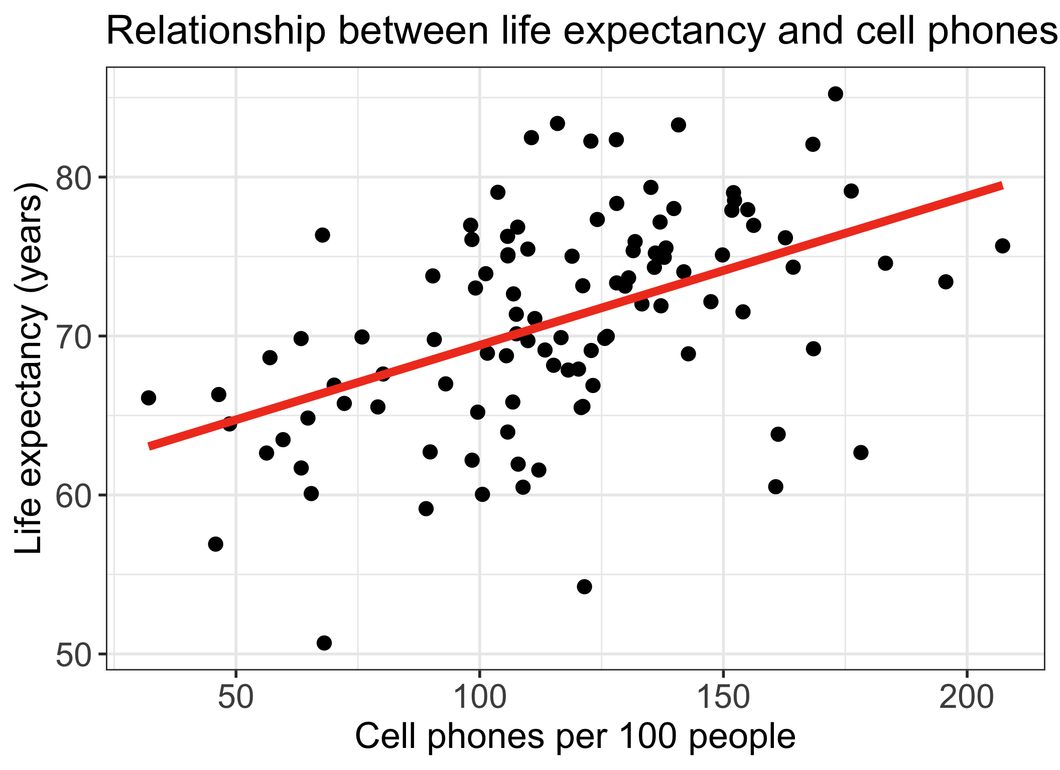
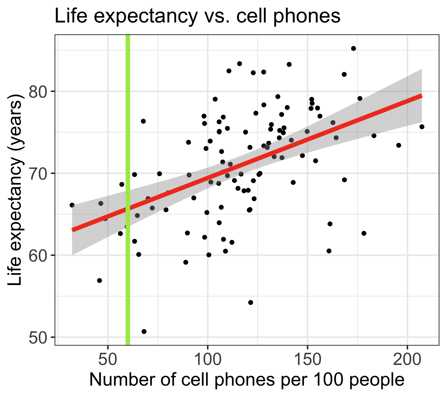
Let’s remind ourselves of the model that we fit last lesson
We fit Gapminder data with cell phones as our independent variable and life expectancy as our dependent variable
We used OLS to find the coefficient estimates of our best-fit line
| term | estimate | std.error | statistic | p.value |
|---|---|---|---|---|
| (Intercept) | 60.04 | 2.06 | 29.21 | 0.00 |
| cell_phones_100 | 0.09 | 0.02 | 5.55 | 0.00 |
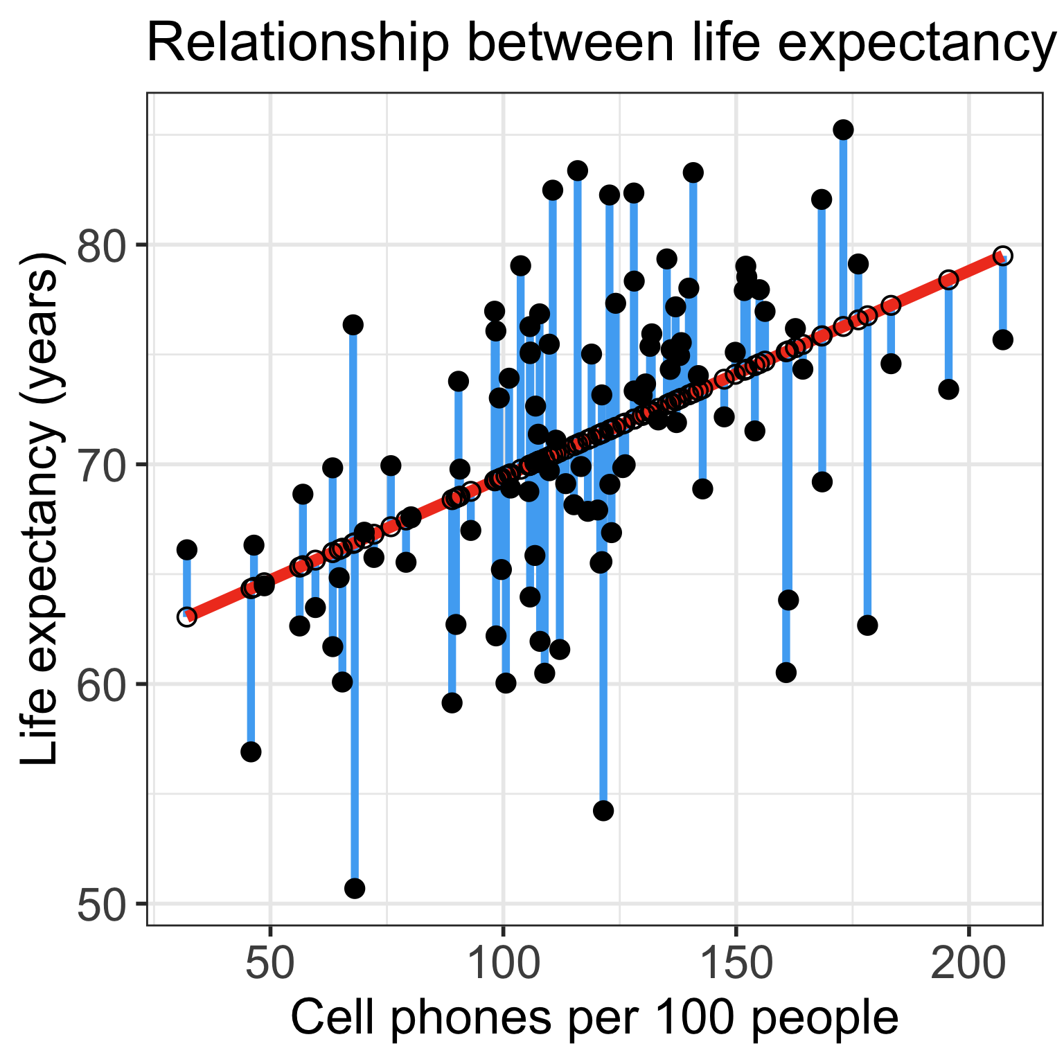
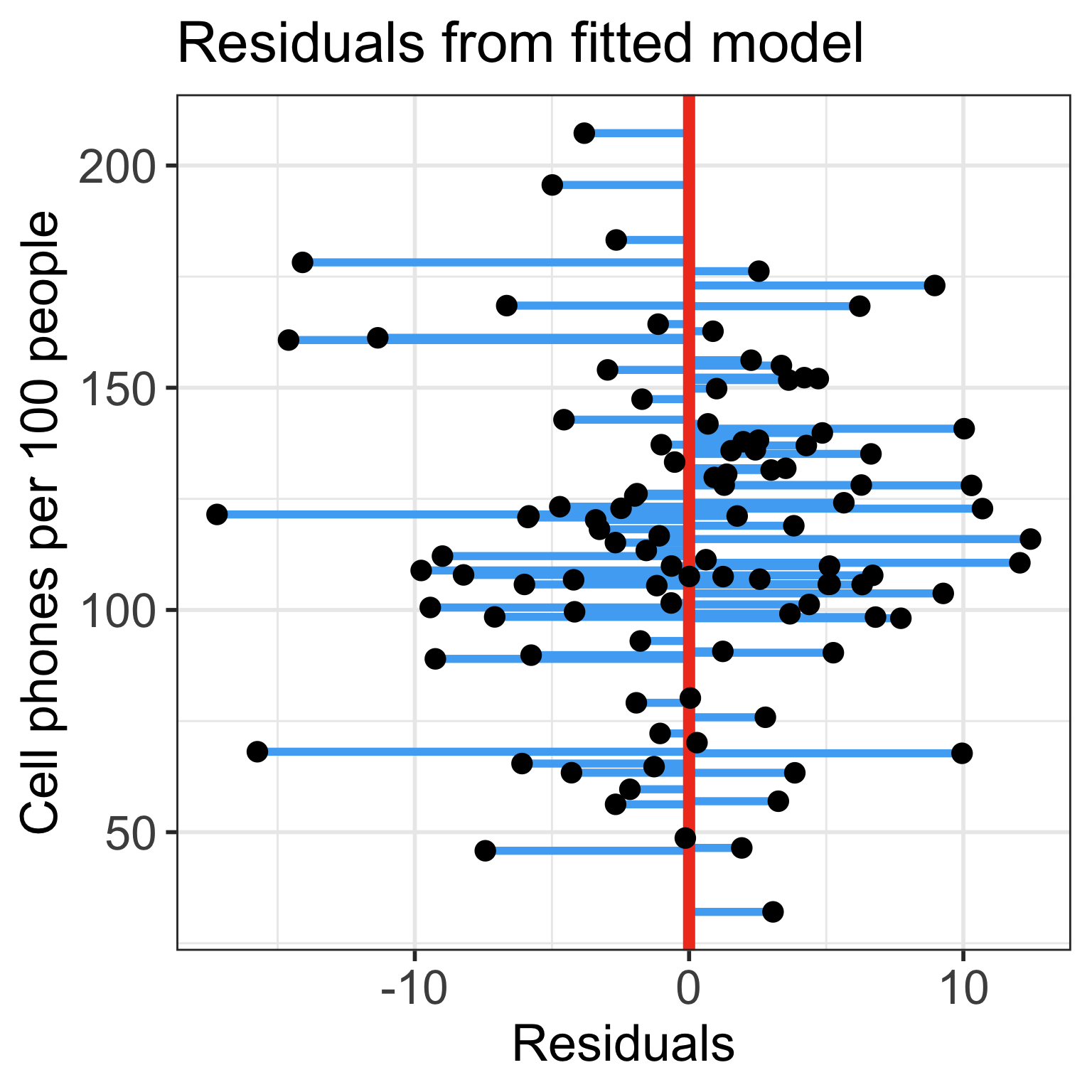
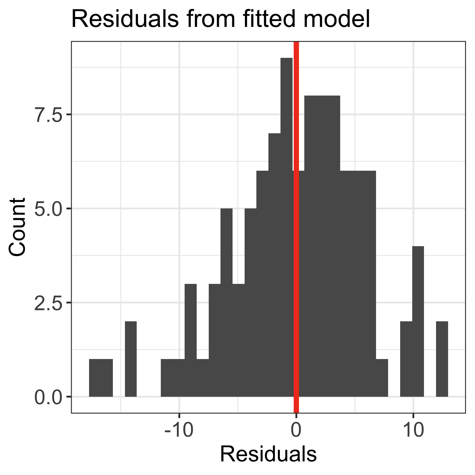
Residuals recap
- Recall our population model residuals are distributed by \(\epsilon \sim N(0, \sigma^2)\)
- And our estimated residuals are \(\widehat\epsilon \sim N(0, \widehat\sigma^2)\)
Standard error of fitted slope \(\widehat\beta_1\)

\[\text{SE}_{\widehat\beta_1} = \frac{\widehat{\sigma}}{s_X\sqrt{n-1}}\]
\(\text{SE}_{\widehat\beta_1}\) is a measure of variability of the estimate \(\widehat\beta_1\)
- \(\widehat{\sigma}\) is the standard deviation of the residuals
- \(s_X\) is the sample standard deviation of the explanatory variable \(X\)
- \(n\) is the sample size, or the number of observations in the model
Calculating standard error for \(\widehat\beta_1\) (1/2)
- Option 1: Calculate using the formula
# A tibble: 1 × 12
  r.squared adj.r.squared sigma statistic     p.value    df logLik   AIC   BIC
      <dbl>         <dbl> <dbl>     <dbl>       <dbl> <dbl>  <dbl> <dbl> <dbl>
1     0.230         0.222  5.96      30.8 0.000000227     1  -335.  677.  685.
# ℹ 3 more variables: deviance <dbl>, df.residual <int>, nobs <int>[1] 5.964089[1] 34.56469[1] 105[1] 0.01691978Calculating standard error for \(\widehat\beta_1\) (2/2)
- Option 2: Use regression table
Mean response/prediction with regression line
Recall the population model:
line + random “noise”
\[Y = \beta_0 + \beta_1 \cdot X + \varepsilon\] with \(\varepsilon \sim N(0,\sigma^2)\)
- When we take the expected value, at a given value \(X^*\), the average/expected response at \(X^*\) is:
\[\widehat{E}[Y|X^*] = \widehat\beta_0 + \widehat\beta_1 X^*\]
- These are the points on the regression line
- The mean responses have variability, and we can calculate a CI for it, for every value of \(X^*\)
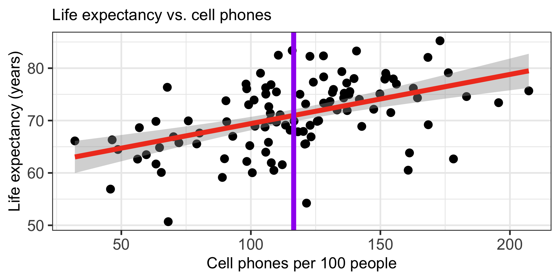
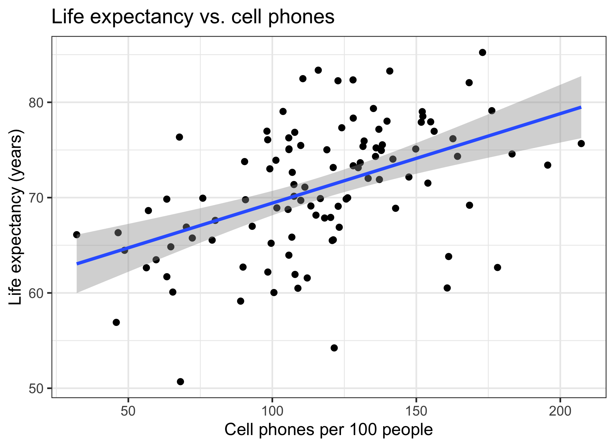
Confidence bands for mean response \(\mu_{Y|X^*}\)
- Often we plot the CI for many values of X, creating confidence bands
- The confidence bands are what ggplot creates when we set
se = TRUEwithingeom_smooth - Think about it: for what values of X are the confidence bands (intervals) narrowest?
Width of confidence bands for mean response \(\mu_{Y|X^*}\)
- For what values of \(X^*\) are the confidence bands (intervals) narrowest? widest?