Code
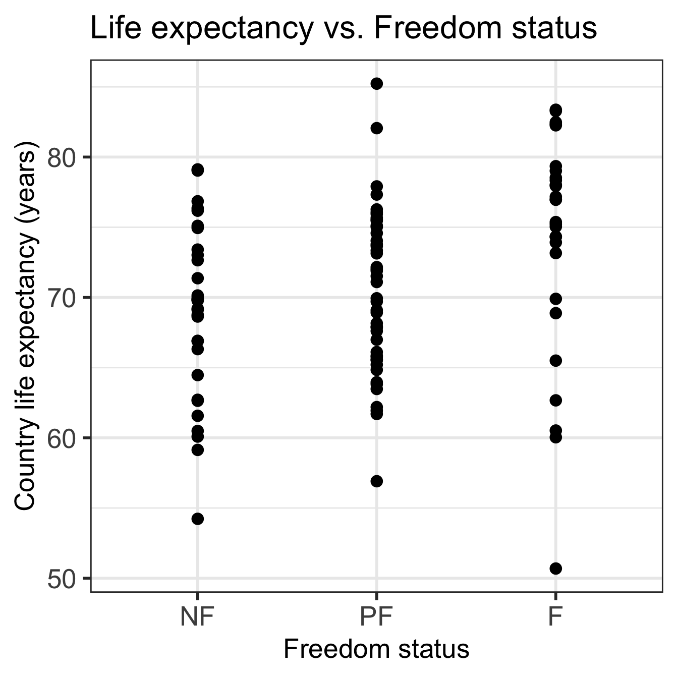
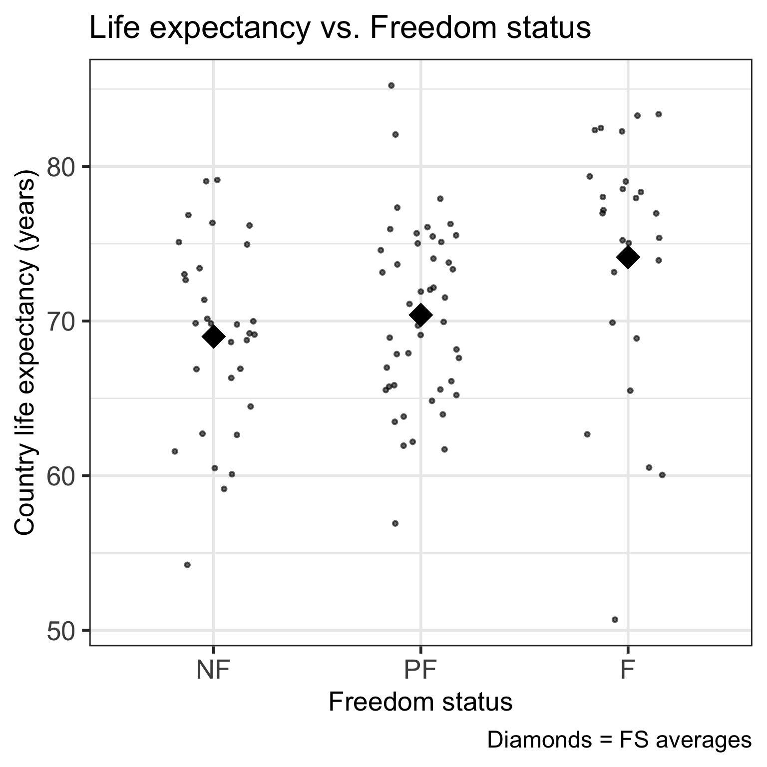
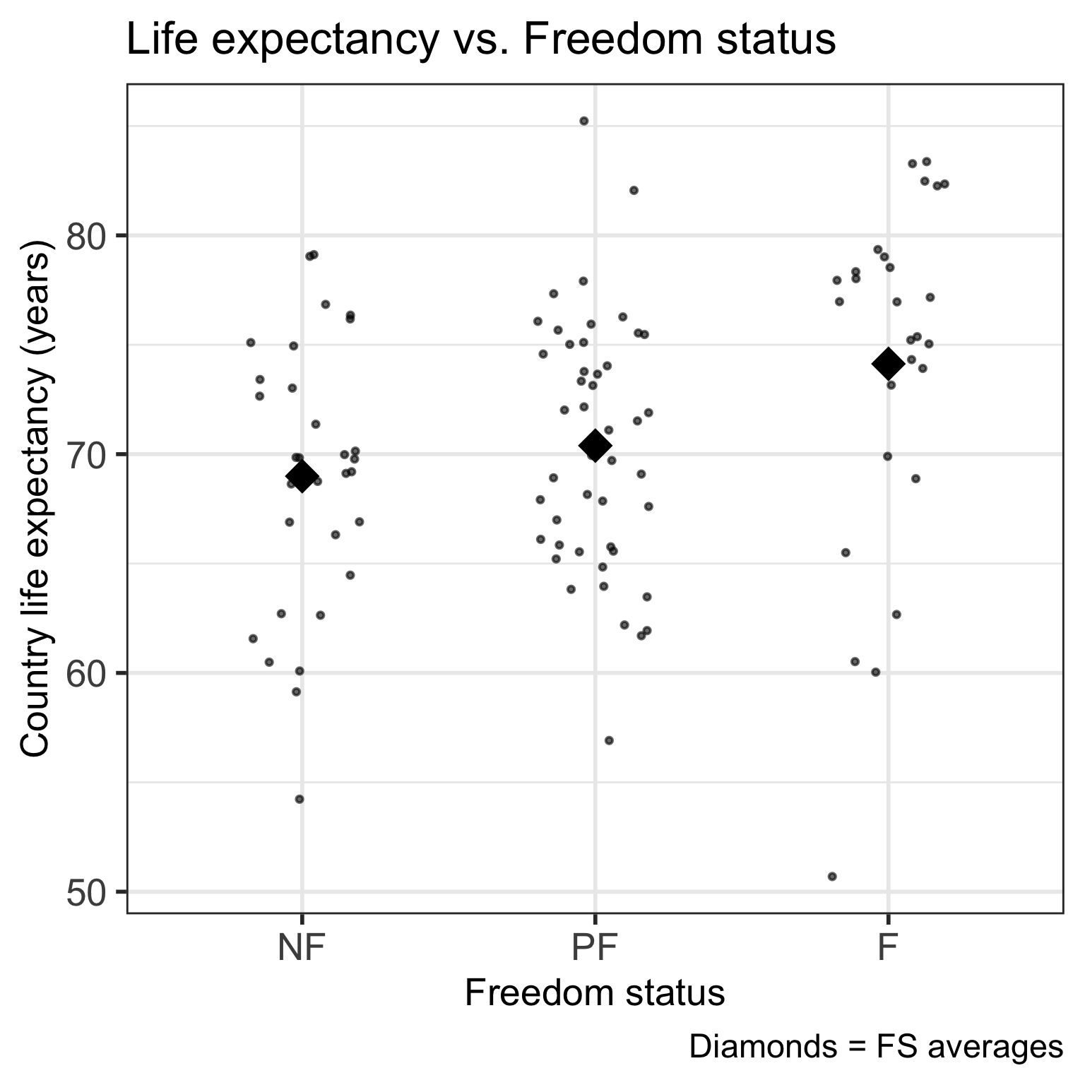
ggplot(gapm, aes(x = fct_reorder(freedom_status, fs_order), y = life_exp)) +
  geom_point() +
  labs(x = "Freedom status",
       y = "Country life expectancy (years)",
       title = "Life expectancy vs. Freedom status") +
  theme(axis.title = element_text(size = 20),
        axis.text = element_text(size = 20),
        title = element_text(size = 20))