Lesson 6: SLR: More inference
2026-01-28
Process of regression data analysis

![]()
![]()
Model Selection
Building a model
Selecting variables
Prediction vs interpretation
Comparing potential models
Model Fitting
Find best fit line
Using OLS in this class
Parameter estimation
Categorical covariates
Interactions
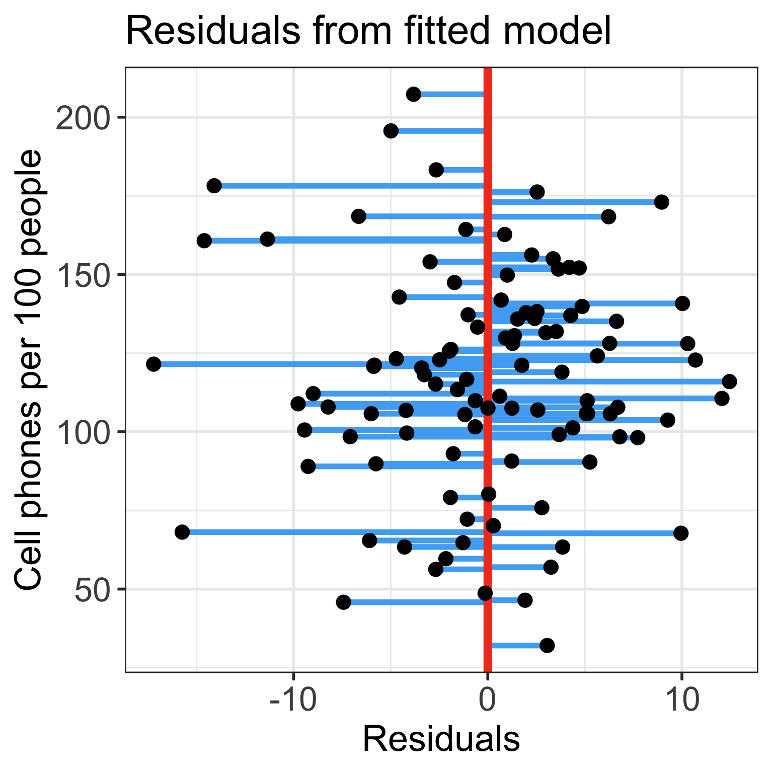
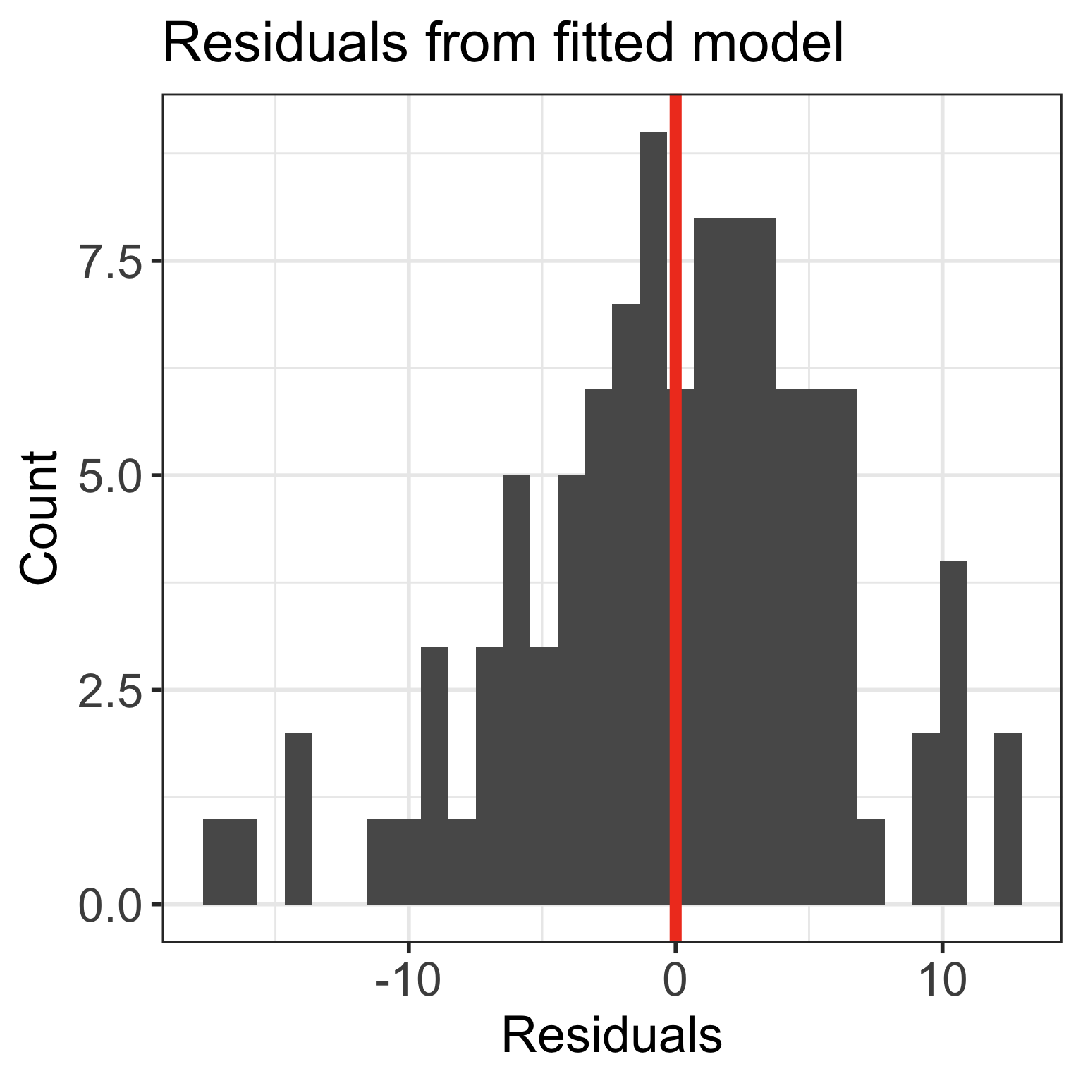
Model Evaluation
- Evaluation of model fit
- Testing model assumptions
- Residuals
- Transformations
- Influential points
- Multicollinearity
Model Use (Inference)
- Inference for coefficients
- Hypothesis testing for coefficients
- Inference for expected \(Y\) given \(X\)
- Prediction of new \(Y\) given \(X\)
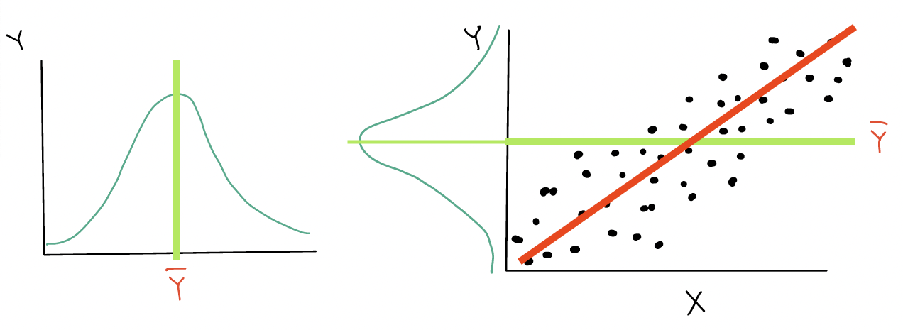
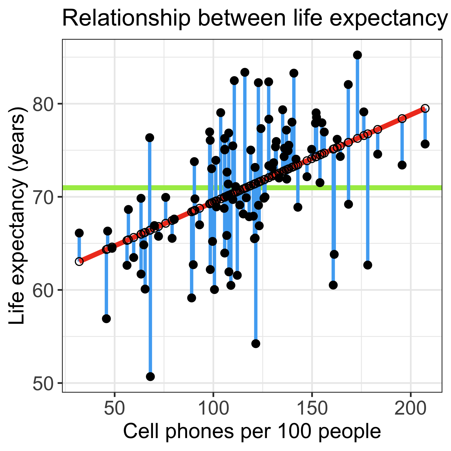
Explained vs. Unexplained Variation
\[ \begin{aligned} Y_i - \overline{Y} & = (Y_i - \widehat{Y}_i) + (\widehat{Y}_i- \overline{Y})\\ \text{Total variation} & = \text{Residual variation after regression} + \text{Variation explained by regression} \end{aligned}\]
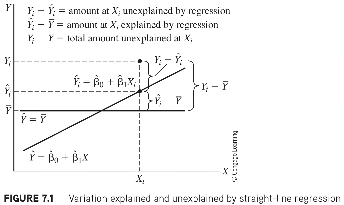
More on the equation
\[Y_i - \overline{Y} = (Y_i - \widehat{Y}_i) + (\widehat{Y}_i- \overline{Y})\]
- \(Y_i - \overline{Y}\) = the deviation of \(Y_i\) around the mean \(\overline{Y}\)
- (the total amount deviation)
- \(Y_i - \widehat{Y}_i\) = the deviation of the observation \(Y\) around the fitted regression line
- (the amount deviation unexplained by the regression at \(X_i\) ).
- \(\widehat{Y_i}- \overline{Y}\) = the deviation of the fitted value \(\widehat{Y}_i\) around the mean \(\overline{Y}\)
- (the amount deviation explained by the regression at \(X_i\) )
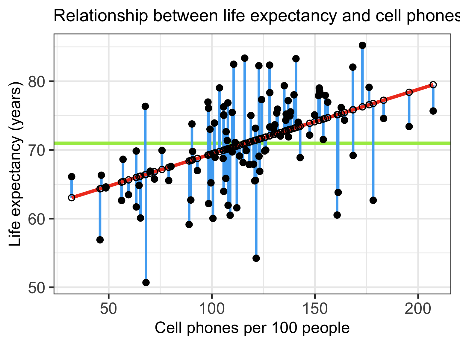
Another way of thinking about the different deviations
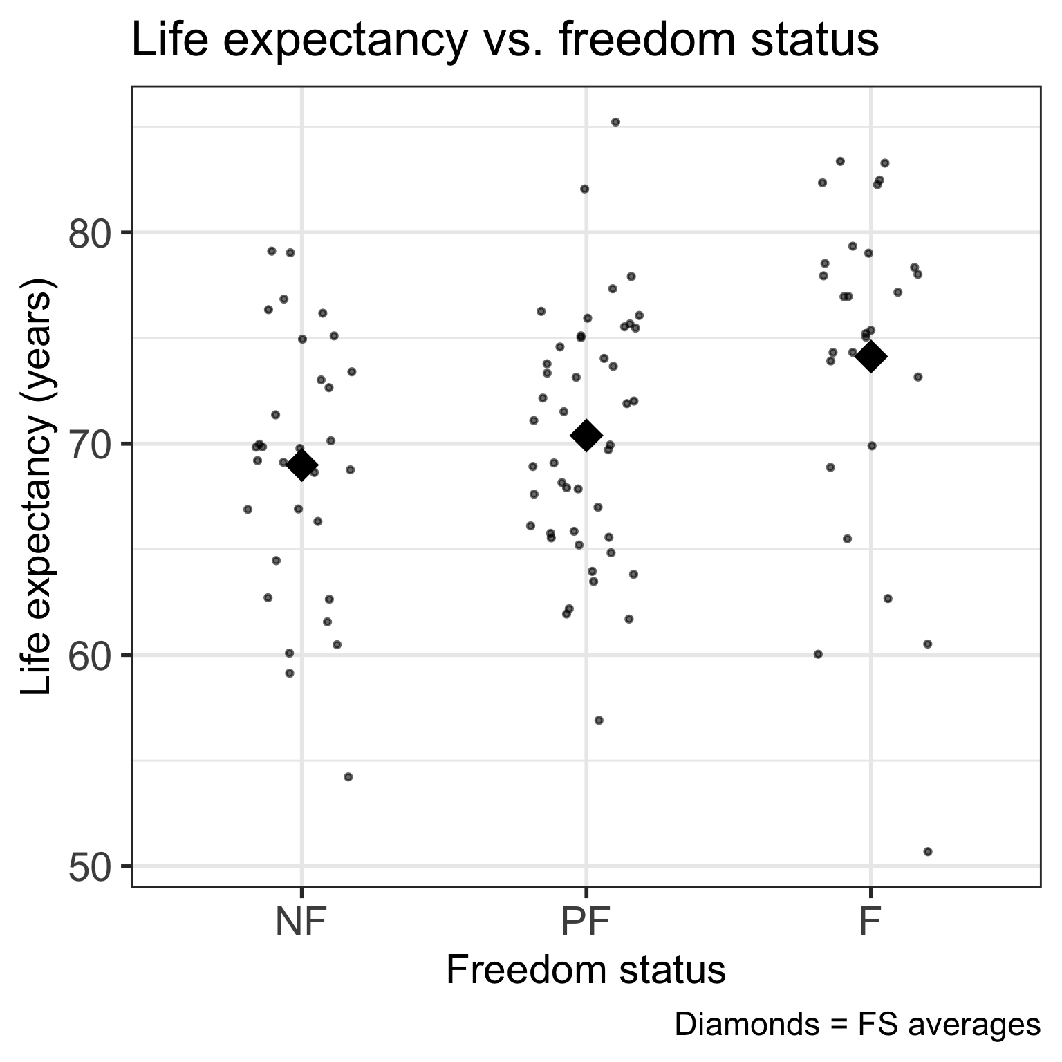
Let’s say we want to test the association between life expectancy and freedom status
\[\begin{aligned} \widehat{\textrm{LE}} = & \widehat\beta_0 + \widehat\beta_1 \cdot I(\text{PF}) + \\ & \widehat\beta_2 \cdot I(\text{F}) \\ \widehat{\textrm{LE}} = & 68.99 + 1.4 \cdot I(\text{PF}) + \\ &5.14 \cdot I(\text{F}) \end{aligned}\]
- We need to figure out if the model with freedom status explains significantly more variation than the model without freedom status!
Correlation coefficient from 511
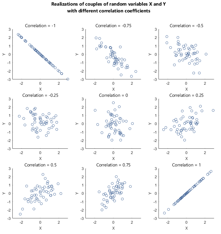
Correlation coefficient \(r\) can tell us about the strength of a relationship between two continuous variables
If \(r = -1\), then there is a perfect negative linear relationship between \(X\) and \(Y\)
If \(r = 1\), then there is a perfect positive linear relationship between \(X\) and \(Y\)
If \(r = 0\), then there is no linear relationship between \(X\) and \(Y\)
Note: All other values of \(r\) tell us that the relationship between \(X\) and \(Y\) is not perfect. The closer \(r\) is to 0, the weaker the linear relationship.
What does \(R^2\) not measure?
\(R^2\) is not a measure of the magnitude of the slope of the regression line
- Example: can have \(R^2 = 1\) for many different slopes!!
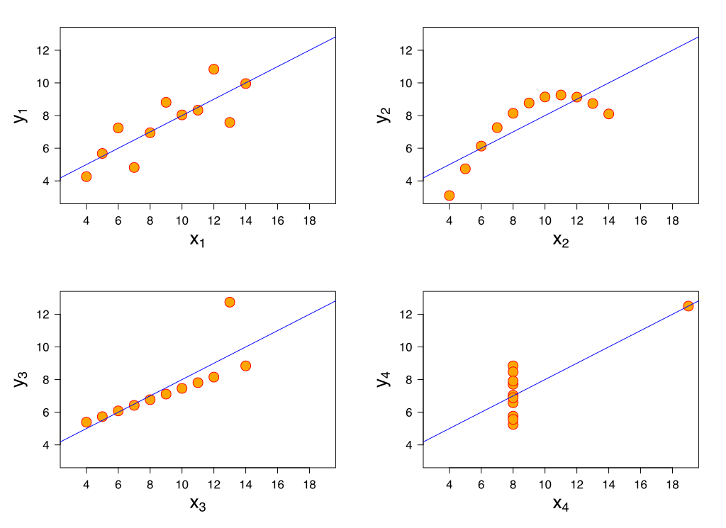
\(R^2\) is not a measure of the appropriateness of the straight-line model
- Example: figure