Lesson 9: Introduction to Multiple Linear Regression (MLR)

Nicky Wakim

2026-02-09

Learning Objectives

1. Understand the population multiple linear regression model through equations.
2. Fit MLR model (in R) with one continuous and one categorical predictor.
3. Interpret MLR coefficient estimates from model with one continuous and one categorical predictor.
4. Fit MLR model (in R) with two continuous predictors.
5. Interpret MLR coefficient estimates from model with two continuous predictors.

Reminder of what we learned in the context of SLR

• SLR helped us establish the foundation for a lot of regression

  • But we do not usually use SLR in analysis

What did we learn in SLR??

Model Fitting

• Ordinary least squares (OLS)
• lm() function in R

Model Use

• Inference for variance of residuals
• Hypothesis testing for coefficients
• Interpreting population coefficient estimates
• Calculated the expected mean for specific \(X\) values
• Interpreted coefficient of determination

Model Evaluation/Diagnostics

• LINE Assumptions
• Influential points
• Data Transformations

Let’s map that to our regression analysis process

Model Selection

• Building a model

• Selecting variables

• Prediction vs interpretation

• Comparing potential models

Model Fitting

• Find best fit line

• Using OLS in this class

• Parameter estimation

• Categorical covariates

• Interactions

Model Evaluation

• Evaluation of model fit
• Testing model assumptions
• Residuals
• Transformations
• Influential points
• Multicollinearity

Model Use (Inference)

• Inference for coefficients
• Hypothesis testing for coefficients

• Inference for expected \(Y\) given \(X\)

Going back to our life expectancy example

• In SLR, we only had one predictor and one outcome in the model:

  • Outcome: Life expectancy = the average number of years a newborn child would live if current mortality patterns were to stay the same.

  • Predictor: Cell phones per 100 people, the number of cell phones per 100 people in a country

• Let’s say many other variables were measured for each country (see codebook)

  • Income levels: Low income, Lower middle income, Upper middle income, High income
  • Vaccination rate: The percentage of one-year-olds who have received at least one of the following vaccinations: BCG, DTP3, HepB3, HIB3, Measles 1st,Measles 2nd, PCV3, Pol3 or RotaC.

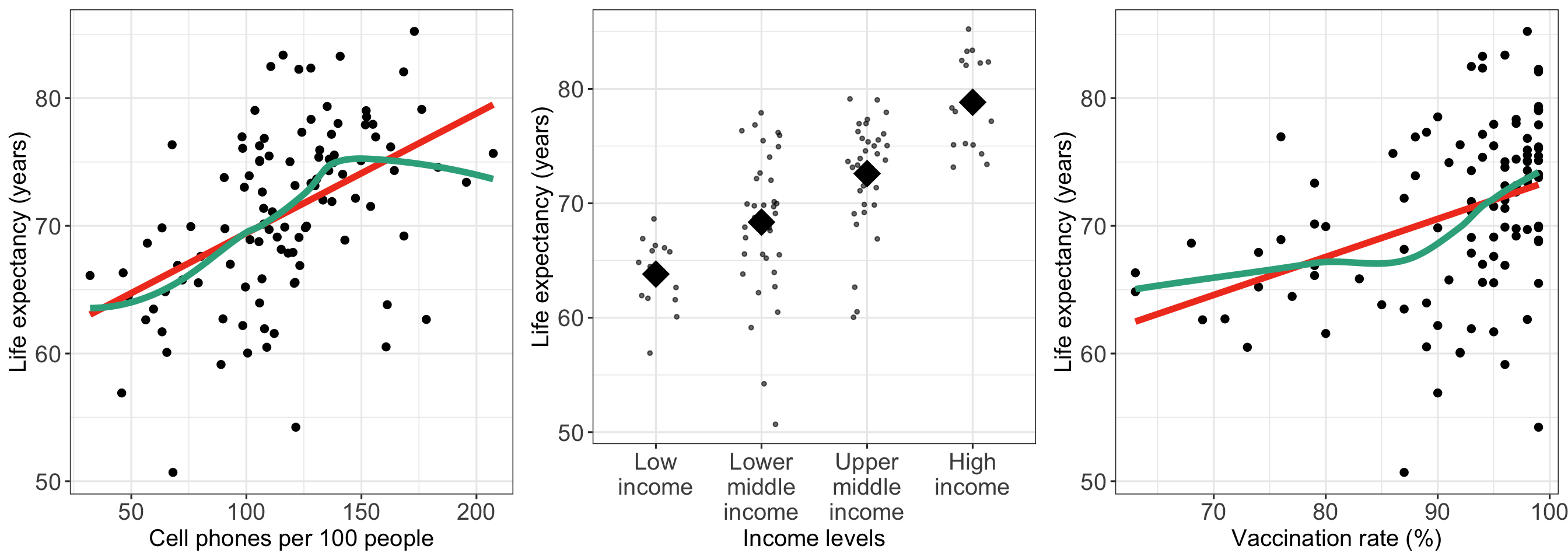
We have seen some work with these variables

• We have looked at some of the “simple” linear regression relationships between life expectancy and these variables (e.g. cell phones, income level, vaccination rate)

Learning Objectives

1. Understand the population multiple linear regression model through equations.

2. Fit MLR model (in R) with one continuous and one categorical predictor.
3. Interpret MLR coefficient estimates from model with one continuous and one categorical predictor.
4. Fit MLR model (in R) with two continuous predictors.
5. Interpret MLR coefficient estimates from model with two continuous predictors.

Simple Linear Regression vs. Multiple Linear Regression

Simple Linear Regression

 

We use one predictor to try to explain the variance of the outcome

\[ Y = \beta_0 + \beta_1 X + \epsilon \]

Multiple Linear Regression

 

We use multiple predictors to try to explain the variance of the outcome

\[ Y = \beta_0 + \beta_1 X_1 + \beta_2 X_2 + ... + \beta_{k}X_{k}+ \epsilon \]

 

• Has \(k+1\) total coefficients (including intercept) for \(k\) predictors/covariates
• Sometimes referred to as multivariable linear regression, but never multivariate

 

• The models have similar “LINE” assumptions and follow the same general diagnostic procedure

Population multiple regression model

\[Y = \beta_0 + \beta_1 X_1 + \beta_2 X_2+ \ldots + \beta_k X_k + \epsilon\]

or on the individual (observation) level:

\[y_i = \beta_0 + \beta_1 x_{i1} + \beta_2 x_{i2}+ \ldots + \beta_k x_{ik} + \epsilon_i,\ \ \text{for}\ i = 1, 2, \ldots, n\]

Observable sample data

• \(Y\) is our dependent variable

  • Aka outcome or response variable

• \(X_1, X_2, \ldots, X_k\) are our \(k\) independent variables

  • Aka predictors or covariates

Unobservable population parameters

• \(\beta_0, \beta_1, \beta_2, \ldots, \beta_k\) are unknown population parameters
  • From our sample, we find the population parameter estimates: \(\widehat{\beta}_0, \widehat{\beta}_1, \widehat{\beta}_2, \ldots, \widehat{\beta}_k\)
• \(\epsilon\) is the random error
  • And is still normally distributed
  • \(\epsilon \sim N(0, \sigma^2)\) where \(\sigma^2\) is the population parameter of the variance

Learning Objectives

1. Understand the population multiple linear regression model through equations.

2. Fit MLR model (in R) with one continuous and one categorical predictor.

3. Interpret MLR coefficient estimates from model with one continuous and one categorical predictor.
4. Fit MLR model (in R) with two continuous predictors.
5. Interpret MLR coefficient estimates from model with two continuous predictors.

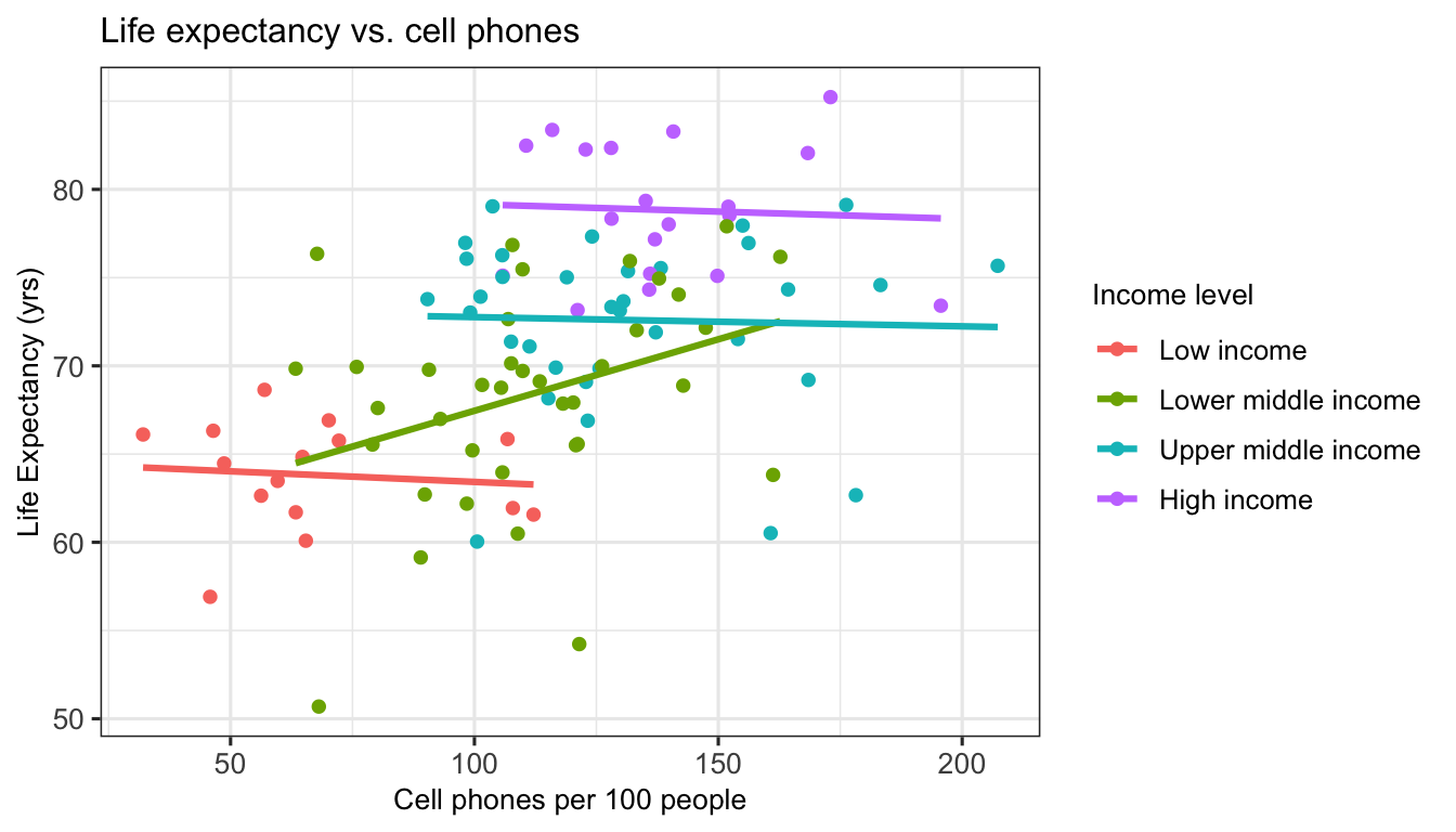
Visualize relationship: life expectancy, cell phones, and income level

Poll Everywhere Question 1

How can we model life expectancy with cell phones and income level?

Simple linear regression population model

\[\begin{aligned} \text{LE} & = \beta_0 + \beta_1 \text{CP} + \epsilon \end{aligned}\]

Multiple linear regression population model (with added income level)

\[\begin{aligned} \text{LE} = & \beta_0 + \beta_1 \text{CP} + \beta_2 I(IL = \text{``Lower middle"}) + \\ & \beta_3 I(IL = \text{``Upper middle"}) + \beta_2 I(IL = \text{``High"}) + \epsilon \end{aligned}\]

How do we fit a multiple linear regression model in R?

New population model for example:

\[\text{LE} = \beta_0 + \beta_1 \text{CP} + \beta_2 I(IL = \text{``Lower middle"}) + \beta_3 I(IL = \text{``Upper middle"}) + \beta_2 I(IL = \text{``High"}) + \epsilon \]

mr1 <- gapm %>% lm(formula = life_exp ~ cell_phones_100 + income_level_4)
tidy(mr1, conf.int=T) %>% gt() %>% tab_options(table.font.size = 35) %>% fmt_number(decimals = 3)

term	estimate	std.error	statistic	p.value	conf.low	conf.high
(Intercept)	62.254	1.792	34.735	0.000	58.698	65.810
cell_phones_100	0.023	0.019	1.239	0.218	−0.014	0.060
income_level_4Lower middle income	3.518	1.720	2.046	0.043	0.106	6.930
income_level_4Upper middle income	7.293	1.946	3.748	0.000	3.432	11.153
income_level_4High income	13.340	2.176	6.131	0.000	9.024	17.656

Fitted multiple regression model:

\[\begin{aligned} \widehat{\text{LE}} = & \widehat{\beta}_0 + \widehat{\beta}_1 \text{CP} + \widehat{\beta}_2 I(IL = \text{``Lower middle"}) + \widehat{\beta}_3 I(IL = \text{``Upper middle"}) + \widehat{\beta}_2 I(IL = \text{``High"}) \\ \widehat{\text{LE}} = & 62.25 + 0.023 \ \text{CP} + 3.52\ I(IL = \text{``Lower middle"}) + 7.29\ I(IL = \text{``Upper middle"}) + \\ & 13.34\ I(IL = \text{``High"}) \end{aligned}\]

Learning Objectives

1. Understand the population multiple linear regression model through equations.
2. Fit MLR model (in R) with one continuous and one categorical predictor.

3. Interpret MLR coefficient estimates from model with one continuous and one categorical predictor.

4. Fit MLR model (in R) with two continuous predictors.
5. Interpret MLR coefficient estimates from model with two continuous predictors.

Interpreting the estimated population coefficients

• For a fitted model: \[\widehat{Y} = \widehat{\beta}_0 + \widehat{\beta}_1 X_1 + \widehat{\beta}_2 I(X_2=\text{``cat 2"}) + \widehat{\beta}_3 I(X_2=\text{``cat 3"})\]
  • Where \(X_1\) is continuous variable and \(X_2\) is categorical with 3 categories

General interpretation for \(\widehat{\beta}_0\)

The expected \(Y\)-variable is (\(\widehat\beta_0\) units) when the \(X_1\)-variable is 0 \(X_1\)-units and \(X_2\)-variable is reference group (cat 1) (95% CI: LB, UB).

General interpretation for \(\widehat{\beta}_1\)

For every increase of 1 \(X_1\)-unit in the \(X_1\)-variable, adjusting/controlling for \(X_2\)-variable, there is an expected increase/decrease of \(|\widehat\beta_1|\) units in the \(Y\)-variable (95%: LB, UB).

General interpretation for \(\widehat{\beta}_2\)

Adjusting/controlling for \(X_1\)-variable, the difference in mean \(Y\)-variable comparing \(X_2\)-variable in category 2 to the reference group (cat 1) is \(|\widehat\beta_2|\) units (95%: LB, UB).

Interpreting the estimated population coefficient: \(\widehat{\beta}_0\)

• For an estimated model:

\[\widehat{Y} = \widehat{\beta}_0 + \widehat{\beta}_1 X_1 + \widehat{\beta}_2 I(X_2=\text{``cat 2"}) + \widehat{\beta}_3 I(X_2=\text{``cat 3"})\]

• We want to get to a statement with \(\widehat{\beta}_0\) alone: \[\begin{aligned} \widehat{Y} = &\widehat{\beta}_0 + \widehat{\beta}_1 0 + \widehat{\beta}_2 0 + \widehat{\beta}_3 0\\ \widehat{Y} = &\widehat{\beta}_0 \\ \end{aligned}\]

Interpretation: The expected \(Y\)-variable is (\(\widehat\beta_0\) units) when the \(X_1\)-variable is 0 \(X_1\)-units and \(X_2\)-variable is reference group (cat 1) (95% CI: LB, UB).

Interpreting the estimated population coefficient: \(\widehat{\beta}_1\)

• We will use: \(x_{1a}\) and \(x_{1b} = x_{1a} + 1\), with the implication that \(\Delta{x_1} = x_{1b} - x_{1a} = 1\)

• Our goal is to get to a statement with \(\widehat{\beta}_1\) alone:

\[\begin{aligned} \widehat{Y}|x_{1a} = &\widehat{\beta}_0 + \widehat{\beta}_1 x_{1a} + \widehat{\beta}_2 I(X_2=\text{``cat 2"}) + \widehat{\beta}_3 I(X_2=\text{``cat 3"})\\ \widehat{Y}|x_{1b} = &\widehat{\beta}_0 + \widehat{\beta}_1 x_{1b} + \widehat{\beta}_2 I(X_2=\text{``cat 2"}) + \widehat{\beta}_3 I(X_2=\text{``cat 3"})\\ \widehat{Y}|x_{1b} - \widehat{Y}|x_{1a} = & \bigg[\widehat{\beta}_0 + \widehat{\beta}_1 x_{1b} + \widehat{\beta}_2 I(X_2=\text{``cat 2"}) + \widehat{\beta}_3 I(X_2=\text{``cat 3"})\bigg] \\ &- \bigg[\widehat{\beta}_0 + \widehat{\beta}_1 x_{1a} + \widehat{\beta}_2 I(X_2=\text{``cat 2"}) + \widehat{\beta}_3 I(X_2=\text{``cat 3"})\bigg] \\ \widehat{Y}|x_{1b} - \widehat{Y}|x_{1a} = & \widehat{\beta}_1 x_{1b} - \widehat{\beta}_1 x_{1a}\\ \widehat{Y}|x_{1b} - \widehat{Y}|x_{1a} = & \widehat{\beta}_1 (x_{1b} - x_{1a})\\ \widehat{Y}|x_{1b} - \widehat{Y}|x_{1a} = & \widehat{\beta}_1\\ \end{aligned}\]

 

As long as \(X_2\) is the category (aka adjusting or controlling for \(X_2\)), then any terms with \(X_2\) will cancel out

Interpretation: For every increase of 1 \(X_1\)-unit in the \(X_1\)-variable, adjusting/controlling for \(X_2\)-variable, there is an expected increase/decrease of \(|\widehat\beta_1|\) units in the \(Y\)-variable (95%: LB, UB).

Interpreting the estimated population coefficient: \(\widehat{\beta}_2\)

• We can so the same for \(X_2\): \(x_{2a}\) is the reference group and \(x_{2b}\) is category 2

• Our goal is to get to a statement with \(\widehat{\beta}_2\) alone:

\[\begin{aligned} \widehat{Y}|x_{2a} = &\widehat{\beta}_0 + \widehat{\beta}_1 X_1 + \widehat{\beta}_2 \times 0 + \widehat{\beta}_3 \times 0\\ \widehat{Y}|x_{2b} = &\widehat{\beta}_0 + \widehat{\beta}_1 X_1 + \widehat{\beta}_2 \times 1 + \widehat{\beta}_3 \times 0\\ \widehat{Y}|x_{2b} - \widehat{Y}|x_{2a} = & \bigg[\widehat{\beta}_0 + \widehat{\beta}_1 X_1 + \widehat{\beta}_2 \bigg] - \bigg[\widehat{\beta}_0 + \widehat{\beta}_1 X_1\bigg] \\ \widehat{Y}|x_{2b} - \widehat{Y}|x_{2a} = & \widehat{\beta}_2\\ \end{aligned}\]

 

As long as \(X_1\) is the same value (aka adjusting or controlling for \(X_1\)), then the two \(\widehat{\beta}_1X_1\) terms will cancel out

Interpretation: Adjusting/controlling for \(X_1\)-variable, the difference in mean \(Y\)-variable comparing \(X_2\)-variable in category 2 to the reference group (cat 1) is \(|\widehat\beta_2|\) units (95%: LB, UB).

What do the fitted regression lines look like?

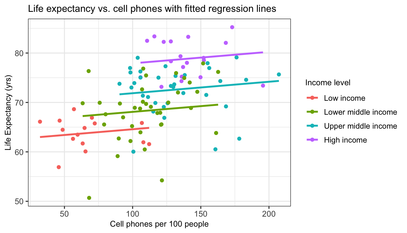
Poll Everywhere Question 2

Getting these interpretations from our regression table

Fitted multiple regression model:

\[\begin{aligned} \widehat{\text{LE}} = & \widehat{\beta}_0 + \widehat{\beta}_1 \text{CP} + \widehat{\beta}_2 I(IL = \text{``Lower middle"}) + \widehat{\beta}_3 I(IL = \text{``Upper middle"}) + \widehat{\beta}_2 I(IL = \text{``High"}) \\ \widehat{\text{LE}} = & 62.25 + 0.023 \ \text{CP} + 3.52\ I(IL = \text{``Lower middle"}) + 7.29\ I(IL = \text{``Upper middle"}) + \\ & 13.34\ I(IL = \text{``High"}) \end{aligned}\]

Interpretation for \(\widehat{\beta}_0\)

The average life expectancy is 62.25 years for a country with 0 cell phones per 100 people and low income status (95% CI: 58.7, 65.81).

Interpretation for \(\widehat{\beta}_1\)

For every increase of 1 cell phone per 100 people, there is an expected increase of 0.023 years in life expectancy (95% CI: -0.014, 0.06), adjusting for income level.

Interpretation for \(\widehat{\beta}_2\)

The difference in average life expectancy comparing lower middle income countries to low income countries is 3.52 years (95% CI: 0.11, 6.93), adjusting for cell phones per 100 people.

Learning Objectives

1. Understand the population multiple linear regression model through equations.
2. Fit MLR model (in R) with one continuous and one categorical predictor.
3. Interpret MLR coefficient estimates from model with one continuous and one categorical predictor.

4. Fit MLR model (in R) with two continuous predictors.

5. Interpret MLR coefficient estimates from model with two continuous predictors.

Can we improve our model by adding food supply as a covariate?

Simple linear regression population model

\[\begin{aligned} \text{LE} = \beta_0 + \beta_1 \text{CP} + \epsilon \end{aligned}\]

Multiple linear regression population model (with added vaccination rate)

\[\begin{aligned} \text{LE} = \beta_0 + \beta_1 \text{CP} + \beta_2 \text{VR} + \epsilon \end{aligned}\]

Visualize relationship: life expectancy, cell phones, and vaccination rate

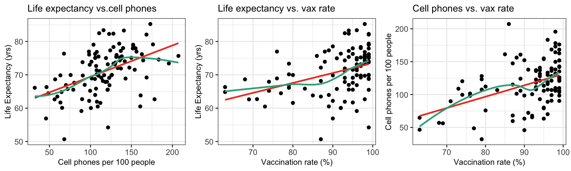
Visualize relationship in 3-D

Relationship with 2D plot with color

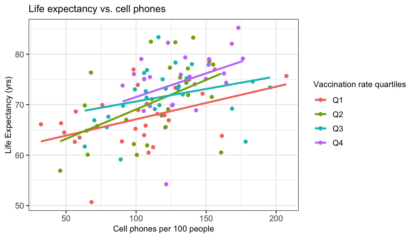
How do we fit a multiple linear regression model in R?

New population model for example:

\[\text{LE} = \beta_0 + \beta_1 \text{CP} + \beta_2 \text{VR} + \epsilon\]

# Fit regression model:
mr1 <- gapm %>% 
  lm(formula = life_exp ~ cell_phones_100 + vax_rate)
tidy(mr1, conf.int=T) %>% gt() %>% tab_options(table.font.size = 35) %>% fmt_number(decimals = 3)

term	estimate	std.error	statistic	p.value	conf.low	conf.high
(Intercept)	46.833	6.042	7.751	0.000	34.848	58.818
cell_phones_100	0.075	0.018	4.074	0.000	0.039	0.112
vax_rate	0.168	0.073	2.318	0.022	0.024	0.312

Fitted multiple regression model:

\[\begin{aligned} \widehat{\text{LE}} &= \widehat{\beta}_0 + \widehat{\beta}_1 \text{CP} + \widehat{\beta}_2 \text{VR} \\ \widehat{\text{LE}} &= 46.833 + 0.075 \ \text{CP} + 0.168\ \text{VR} \end{aligned}\]

Visualize the fitted multiple regression model

• The fitted model equation \[\widehat{Y} = \widehat{\beta}_0 + \widehat{\beta}_1 \cdot X_1 + \widehat{\beta}_2 \cdot X_2\] has three variables (\(Y, X_1,\) and \(X_2\)) and thus we need 3 dimensions to plot it

 

• Instead of a regression line, we get a regression plane
  • See code in .qmd- file. I hid it from view in the html file.

Regression lines for varying values of food supply

\[\begin{aligned} \widehat{\text{LE}} &= \widehat{\beta}_0 + \widehat{\beta}_1 \text{CP} + \widehat{\beta}_2 \text{VR} \\ \widehat{\text{LE}} &= 46.833 + 0.075 \ \text{CP} + 0.168\ \text{VR} \end{aligned}\]

• Note: when the vaccination rate is held constant but cell phones varies…
  • then the outcome values change along a line
• Different values of vaccination rate give different lines
  • The intercepts change, but
  • the slopes stay the same (parallel lines)

(mr1_2d = ggPredict(mr1, interactive = T))

How do we calculate the regression line for 80% vaccination rate?

 

\[\begin{aligned} \widehat{\text{LE}} &= 46.833 + 0.075 \ \text{CP} + 0.168\ \text{VR}\\ \widehat{\text{LE}} &= 46.833 + 0.075 \ \text{CP} + 0.168\cdot 80\\ \widehat{\text{LE}} &= 46.833 + 0.075 \ \text{CP} + 13.463 \\ \widehat{\text{LE}} &= 60.297 + 0.075 \ \text{CP} \end{aligned}\]

(mr1_2d = ggPredict(mr1, interactive = T))

Poll Everwhere Question 3

Learning Objectives

1. Understand the population multiple linear regression model through equations.
2. Fit MLR model (in R) with one continuous and one categorical predictor.
3. Interpret MLR coefficient estimates from model with one continuous and one categorical predictor.
4. Fit MLR model (in R) with two continuous predictors.

5. Interpret MLR coefficient estimates from model with two continuous predictors.

Interpreting the estimated population coefficients

• For a population model: \[Y = \beta_0 + \beta_1 X_1 + \beta_2 X_2+ \epsilon\]
  • Where \(X_1\) and \(X_2\) are continuous variables
  • No need to specify \(Y\) because it required to be continuous in linear regression

General interpretation for \(\widehat{\beta}_0\)

The expected \(Y\)-variable is (\(\widehat\beta_0\) units) when the \(X_1\)-variable is 0 \(X_1\)-units and \(X_2\)-variable is 0 \(X_1\)-units (95% CI: LB, UB).

General interpretation for \(\widehat{\beta}_1\)

For every increase of 1 \(X_1\)-unit in the \(X_1\)-variable, adjusting/controlling for \(X_2\)-variable, there is an expected increase/decrease of \(|\widehat\beta_1|\) units in the \(Y\)-variable (95%: LB, UB).

General interpretation for \(\widehat{\beta}_2\)

For every increase of 1 \(X_2\)-unit in the \(X_2\)-variable, adjusting/controlling for \(X_1\)-variable, there is an expected increase/decrease of \(|\widehat\beta_2|\) units in the \(Y\)-variable (95%: LB, UB).

Interpreting the estimated population coefficient: \(\widehat{\beta}_0\)

• For an estimated model: \(\widehat{Y} = \widehat{\beta}_0 + \widehat{\beta}_1 X_2 + \widehat{\beta}_2 X_2\)

\[\begin{aligned} \widehat{Y} = &\widehat{\beta}_0 + \widehat{\beta}_1 0 + \widehat{\beta}_2 0\\ \widehat{Y} = &\widehat{\beta}_0 \\ \end{aligned}\]

Interpretation: The expected \(Y\)-variable is (\(\widehat\beta_0\) units) when the \(X_1\)-variable is 0 \(X_1\)-units and \(X_2\)-variable is 0 \(X_1\)-units (95% CI: LB, UB).

Interpreting the estimated population coefficient: \(\widehat{\beta}_1\)

• We will use: \(x_{1a}\) and \(x_{1b} = x_{1a} + 1\), with the implication that \(\Delta{x_1} = x_{1b} - x_{1a} = 1\)

• Our goal is to get to a statement with \(\widehat{\beta}_1\) alone:

\[\begin{aligned} \widehat{Y}|x_{1a} = &\widehat{\beta}_0 + \widehat{\beta}_1 x_{1a} + \widehat{\beta}_2 X_2\\ \widehat{Y}|x_{1b} = &\widehat{\beta}_0 + \widehat{\beta}_1 x_{1b} + \widehat{\beta}_2 X_2\\ \widehat{Y}|x_{1b} - \widehat{Y}|x_{1a} = & \bigg[\widehat{\beta}_0 + \widehat{\beta}_1 x_{1b} + \widehat{\beta}_2 X_2\bigg] - \bigg[\widehat{\beta}_0 + \widehat{\beta}_1 x_{1a} + \widehat{\beta}_2 X_2\bigg] \\ \widehat{Y}|x_{1b} - \widehat{Y}|x_{1a} = & \widehat{\beta}_1 x_{1b} - \widehat{\beta}_1 x_{1a}\\ \widehat{Y}|x_{1b} - \widehat{Y}|x_{1a} = & \widehat{\beta}_1 (x_{1b} - x_{1a})\\ \widehat{Y}|x_{1b} - \widehat{Y}|x_{1a} = & \widehat{\beta}_1\\ \end{aligned}\]

 

As long as \(X_2\) is the same value (aka adjusting or controlling for \(X_2\)), then the two \(\widehat{\beta}_2X_2\) terms will cancel out

Interpretation: For every increase of 1 \(X_1\)-unit in the \(X_1\)-variable, adjusting/controlling for \(X_2\)-variable, there is an expected increase/decrease of \(|\widehat\beta_1|\) units in the \(Y\)-variable (95%: LB, UB).

Interpreting the estimated population coefficient: \(\widehat{\beta}_2\)

• We can so the same for \(X_2\): \(x_{2a}\) and \(x_{2b} = x_{2a} + 1\), with the implication that \(\Delta{x_2} = x_{2b} - x_{2a} = 1\)

• Our goal is to get to a statement with \(\widehat{\beta}_2\) alone:

\[\begin{aligned} \widehat{Y}|x_{2a} = &\widehat{\beta}_0 + \widehat{\beta}_1 X_1 + \widehat{\beta}_2 x_{2a}\\ \widehat{Y}|x_{2b} = &\widehat{\beta}_0 + \widehat{\beta}_1 X_1 + \widehat{\beta}_2 x_{2b}\\ \widehat{Y}|x_{2b} - \widehat{Y}|x_{2a} = & \bigg[\widehat{\beta}_0 + \widehat{\beta}_1 X_1 + \widehat{\beta}_2 x_{2b} \bigg] - \bigg[\widehat{\beta}_0 + \widehat{\beta}_1 X_1 + \widehat{\beta}_2 x_{2a}\bigg] \\ \widehat{Y}|x_{2b} - \widehat{Y}|x_{2a} = & \widehat{\beta}_2 x_{2b} - \widehat{\beta}_2 x_{2a}\\ \widehat{Y}|x_{2b} - \widehat{Y}|x_{2a} = & \widehat{\beta}_2 (x_{2b} - x_{2a})\\ \widehat{Y}|x_{2b} - \widehat{Y}|x_{2a} = & \widehat{\beta}_2\\ \end{aligned}\]

 

As long as \(X_1\) is the same value (aka adjusting or controlling for \(X_1\)), then the two \(\widehat{\beta}_1X_1\) terms will cancel out

Interpretation: For every increase of 1 \(X_2\)-unit in the \(X_2\)-variable, adjusting/controlling for \(X_1\)-variable, there is an expected increase/decrease of \(|\widehat\beta_2|\) units in the \(Y\)-variable (95%: LB, UB).

Poll Everywhere Question 4

Getting these interpretations from our regression table

We fit the regression model in R and printed the regression table:

mr1 <- lm(life_exp ~ cell_phones_100 + vax_rate, 
          data = gapm)

term	estimate	std.error	statistic	p.value	conf.low	conf.high
(Intercept)	46.833	6.042	7.751	0.000	34.848	58.818
cell_phones_100	0.075	0.018	4.074	0.000	0.039	0.112
vax_rate	0.168	0.073	2.318	0.022	0.024	0.312

Fitted multiple regression model: \(\widehat{\text{LE}} = 46.833 + 0.075 \ \text{CP} + 0.168\ \text{VR}\)

Interpretation for \(\widehat{\beta}_0\)

The average life expectancy is 46.83 years for a country with 0 cell phones per 100 people and 0% vaccination rate (95% CI: 34.85, 58.82).

Interpretation for \(\widehat{\beta}_1\)

For every increase of 1 cell phone per 100 people, there is an expected increase of 0.08 years in a country’s life expectancy (95% CI: 0.04, 0.11), adjusting for vaccination rate.

Interpretation for \(\widehat{\beta}_2\)

For every 1% increase in vaccination rate, there is an expected increase of 0.17 years in a country’s life expectancy (95% CI: 0.02, 0.31), adjusting for cell phones per 100 people.

Extra resources

What we need in our interpretations of coefficients (reference)

• Units of Y

• Units of X

• If discussing intercept: Mean or average or expected before Y

• If discussing coefficient for continuous covariate: Mean or average or expected before difference, increase, or decrease

  • OR: Mean or average or expected before Y
  • NOT: predicted
  • Only need before difference or Y!!

• Confidence interval

• If other covariates in the model

  • Discussing intercept: Must state that variables are equal to 0

    • or at their centered value if centered!

  • Discussing coefficient for covariate: Must state “adjusting for all other variables”, “Controlling for all other variables”, or “Holding all other variables constant”

    • If only one other variable in the model, then replace “all other variables” with the single variable name

Technical side note (not needed in our class)

• The equations for calculating the \(\boldsymbol{\widehat{\beta}}\) values is best done using matrix notation (not required for our class)

• We will be using R to get the coefficients instead of the equation (already did this a few slides back!)

• How we have represented the population regression model: \[Y = \beta_0 + \beta_1 X_1 + \beta_2 X_2+ \ldots + \beta_k X_k + \epsilon\]

• How to represent population model with matrix notation:

\[\begin{aligned} \boldsymbol{Y} &= \boldsymbol{X}\boldsymbol{\beta} + \boldsymbol{\epsilon} \\ \boldsymbol{Y}_{n \times 1}& = \boldsymbol{X}_{n \times (k+1)}\boldsymbol{\beta}_{(k+1)\times 1} + \boldsymbol{\epsilon}_{n \times 1} \end{aligned}\]

• \(\boldsymbol{X}\) is often called the design matrix
  • Each row represents an individual
  • Each column represents a covariate

\[ \boldsymbol{Y} = \left[\begin{array}{c} Y_1 \\ Y_2 \\ \vdots \\ Y_n \end{array} \right]_{n \times 1} \] \[ \boldsymbol{\epsilon} = \left[\begin{array}{c} \epsilon_1 \\ \epsilon_2 \\ \vdots \\ \epsilon_n \end{array} \right]_{n \times 1} \]

\[ \boldsymbol{X} = \left[ \begin{array}{ccccc} 1 & X_{11} & X_{12} & \ldots & X_{1,k} \\ 1 &X_{21} & X_{22} & \ldots & X_{2,k} \\ \vdots&\vdots & \vdots & \ldots & \vdots \\ 1 & X_{n1} & X_{n2} & \ldots & X_{n,k} \end{array} \right]_{n \times (k+1)} \]

\[ \boldsymbol{\beta} = \left[\begin{array}{c} \beta_0 \\ \beta_1\\ \vdots \\ \beta_{k} \end{array} \right]_{(k+1)\times 1} \]