Lesson 12: Interactions, Part 2
Nicky Wakim
2026-02-25
Learning Objectives
Last time:
- Define confounders and effect modifiers, and how they interact with the main relationship we model.
- Interpret the interaction component of a model with a binary categorical covariate and continuous covariate, and how the main variable’s effect changes.
- Interpret the interaction component of a model with a multi-level categorical covariate and continuous covariate, and how the main variable’s effect changes.
This time:
- Interpret the interaction component of a model with two categorical covariates, and how the main variable’s effect changes.
- Interpret the interaction component of a model with two continuous covariates, and how the main variable’s effect changes.
- Report results for a best-fit line (with confidence intervals) at different levels of an effect measure modifier
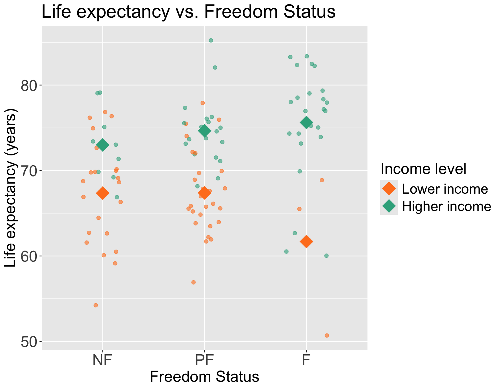
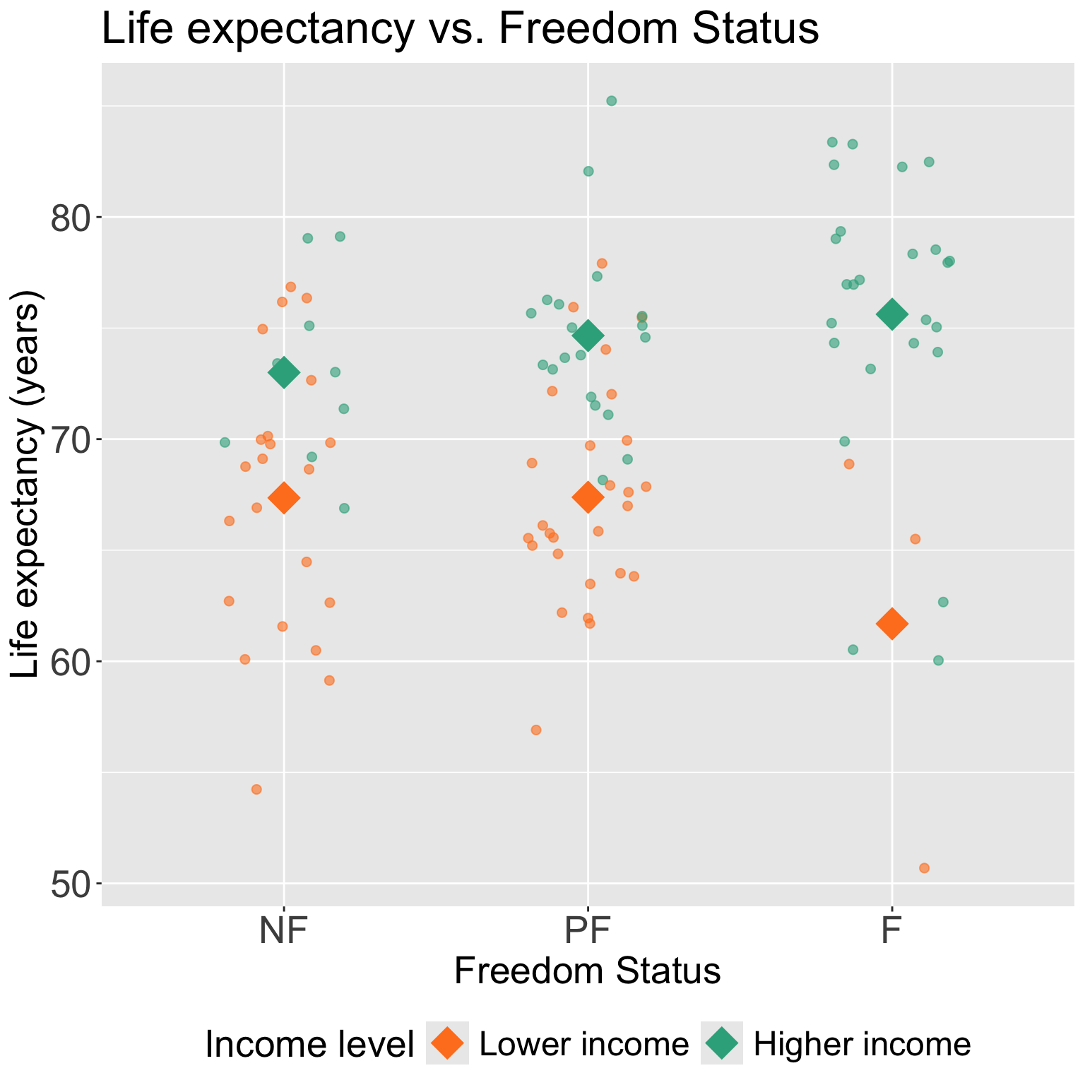
Do we think income level can be an effect modifier for freedom status?
Taking a break from cell phones to demonstrate interactions for two categorical variables
We can start by visualizing the relationship between life expectancy and freedom status by income level
Questions of interest: Does the effect of freedom status on life expectancy differ depending on income level?
- This is the same as: Is income level an effect modifier for freedom status?
Let’s run an interaction model to see!
Model with interaction between a multi-level categorical and binary variables
Model we are fitting:
\[\begin{aligned}LE = &\beta_0 + \beta_1 I(\text{high income}) + \beta_2 I(\text{FS} = \text{PF}) + \beta_3 I(\text{FS} = \text{F}) + \\ & \beta_4 \cdot I(\text{high income}) \cdot I(\text{FS} = \text{PF}) + \beta_5 \cdot I(\text{high income}) \cdot I(\text{FS} = \text{F}) + \epsilon \end{aligned}\]
- \(LE\) as life expectancy
- \(I(\text{high income})\) as indicator of high income
- \(I(\text{FS} = \text{PF})\) and \(I(\text{FS} = \text{F})\) as the indicator for each freedom status
In R:
Displaying the regression table and writing fitted regression equation
| term | estimate | std.error | statistic | p.value | conf.low | conf.high |
|---|---|---|---|---|---|---|
| (Intercept) | 67.355 | 1.179 | 57.126 | 0.000 | 65.015 | 69.695 |
| income_level_2Higher income | 5.645 | 2.188 | 2.580 | 0.011 | 1.303 | 9.987 |
| freedom_statusPF | 0.029 | 1.588 | 0.018 | 0.985 | −3.123 | 3.181 |
| freedom_statusF | −5.665 | 3.404 | −1.664 | 0.099 | −12.419 | 1.089 |
| income_level_2Higher income:freedom_statusPF | 1.633 | 2.744 | 0.595 | 0.553 | −3.813 | 7.078 |
| income_level_2Higher income:freedom_statusF | 8.287 | 4.026 | 2.058 | 0.042 | 0.299 | 16.275 |
\[\begin{aligned} \widehat{LE} = &\widehat\beta_0 + \widehat\beta_1 I(\text{high income}) + \widehat\beta_2 I(\text{FS} = \text{PF}) + \widehat\beta_3 I(\text{FS} = \text{F}) + \\ & \widehat\beta_4 \cdot I(\text{high income}) \cdot I(\text{FS} = \text{PF}) + \widehat\beta_5\cdot I(\text{high income}) \cdot I(\text{FS} = \text{F})\\ \widehat{LE} = & 67.35 + 5.64 \cdot I(\text{high income}) + 0.03 \cdot I(\text{FS} = \text{PF}) -5.67 \cdot I(\text{FS} = \text{F}) + \\ & 1.63 \cdot I(\text{high income}) \cdot I(\text{FS} = \text{PF}) + 8.29\cdot I(\text{high income}) \cdot I(\text{FS} = \text{F})\\ \end{aligned}\]
Poll Everywhere Question 4
Comparing fitted regression means for each freedom status
\[\begin{aligned} \widehat{LE} = &\widehat\beta_0 + \widehat\beta_1 I(\text{high income}) + \widehat\beta_2 I(\text{FS} = \text{PF}) + \widehat\beta_3 I(\text{FS} = \text{F}) + \\ & \widehat\beta_4 \cdot I(\text{high income}) \cdot I(\text{FS} = \text{PF}) + \widehat\beta_5\cdot I(\text{high income}) \cdot I(\text{FS} = \text{F})\\ \widehat{LE} = & 67.35 + 5.64 \cdot I(\text{high income}) + 0.03 \cdot I(\text{FS} = \text{PF}) -5.67 \cdot I(\text{FS} = \text{F}) + \\ & 1.63 \cdot I(\text{high income}) \cdot I(\text{FS} = \text{PF}) + 8.29\cdot I(\text{high income}) \cdot I(\text{FS} = \text{F}) \end{aligned}\]
Not free
\[\begin{aligned} \widehat{LE} = &\widehat\beta_0 + \widehat\beta_1 I(\text{high income}) + \\ & \widehat\beta_2 \cdot 0 + \widehat\beta_3 \cdot 0 + \\ & \widehat\beta_4 \cdot I(\text{high income}) \cdot 0 + \\ & \widehat\beta_5\cdot I(\text{high income}) \cdot 0 \\ \widehat{LE} = &\widehat\beta_0 + \widehat\beta_1 I(\text{high income}) \end{aligned}\]
Partly free
\[\begin{aligned} \widehat{LE} = &\widehat\beta_0 + \widehat\beta_1 I(\text{high income}) + \\ & \widehat\beta_2 \cdot 1 + \widehat\beta_3 \cdot 0 + \\ & \widehat\beta_4 \cdot I(\text{high income}) \cdot 1 + \\ & \widehat\beta_5\cdot I(\text{high income}) \cdot 0 \\ \widehat{LE} = & \big(\widehat\beta_0 + \widehat\beta_2 \big) + \\ & \big(\widehat\beta_1 + \widehat\beta_4 \big) I(\text{high income}) \\ \end{aligned}\]
Free
\[\begin{aligned} \widehat{LE} = &\widehat\beta_0 + \widehat\beta_1 I(\text{high income}) + \\ & \widehat\beta_2 \cdot 1 + \widehat\beta_3 \cdot 0 + \\ & \widehat\beta_4 \cdot I(\text{high income}) \cdot 1 + \\ & \widehat\beta_5\cdot I(\text{high income}) \cdot 0 \\ \widehat{LE} = & \big(\widehat\beta_0 + \widehat\beta_3 \big) + \\ & \big(\widehat\beta_1 + \widehat\beta_5 \big) I(\text{high income}) \\ \end{aligned}\]
Comparing fitted regression means for each income level
\[\begin{aligned} \widehat{LE} = &\widehat\beta_0 + \widehat\beta_1 I(\text{high income}) + \widehat\beta_2 I(\text{FS} = \text{PF}) + \widehat\beta_3 I(\text{FS} = \text{F}) + \\ & \widehat\beta_4 \cdot I(\text{high income}) \cdot I(\text{FS} = \text{PF}) + \widehat\beta_5\cdot I(\text{high income}) \cdot I(\text{FS} = \text{F})\\ \widehat{LE} = & 67.35 + 5.64 \cdot I(\text{high income}) + 0.03 \cdot I(\text{FS} = \text{PF}) -5.67 \cdot I(\text{FS} = \text{F}) + \\ & 1.63 \cdot I(\text{high income}) \cdot I(\text{FS} = \text{PF}) + 8.29\cdot I(\text{high income}) \cdot I(\text{FS} = \text{F}) \end{aligned}\]
For lower income countries: \(I(\text{high income})=0\)
\[ \begin{aligned} \widehat{LE} = &\widehat\beta_0 + \widehat\beta_1 \cdot 0 + \widehat\beta_2 I(\text{FS} = \text{PF}) + \widehat\beta_3 I(\text{FS} = \text{F}) + \\ & \widehat\beta_4 \cdot 0 \cdot I(\text{FS} = \text{PF}) + \widehat\beta_5 \cdot 0 \cdot I(\text{FS} = \text{F})\\ \widehat{LE} = & \widehat\beta_0 + \widehat\beta_2 I(\text{FS} = \text{PF}) + \widehat\beta_3 I(\text{FS} = \text{F}) \\ \end{aligned}\]
For higher income countries: \(I(\text{high income}) =1\)
\[ \begin{aligned} \widehat{LE} = &\widehat\beta_0 + \widehat\beta_1 \cdot 1 + \widehat\beta_2 I(\text{FS} = \text{PF}) + \widehat\beta_3 I(\text{FS} = \text{F}) + \\ & \widehat\beta_4 \cdot 1 \cdot I(\text{FS} = \text{PF}) + \widehat\beta_5 \cdot 1 \cdot I(\text{FS} = \text{F})\\ \widehat{LE} = & \big(\widehat\beta_0 + \widehat\beta_1 \big) + \big(\widehat\beta_2 + \widehat\beta_4 \big) I(\text{FS} = \text{PF}) + \\ & \big(\widehat\beta_3 + \widehat\beta_5 \big) I(\text{FS} = \text{F}) \\ \end{aligned}\]
- Example interpretation: The America’s effect on mean life expectancy increases \(\widehat{\beta}_5\) comparing high income to low income countries.
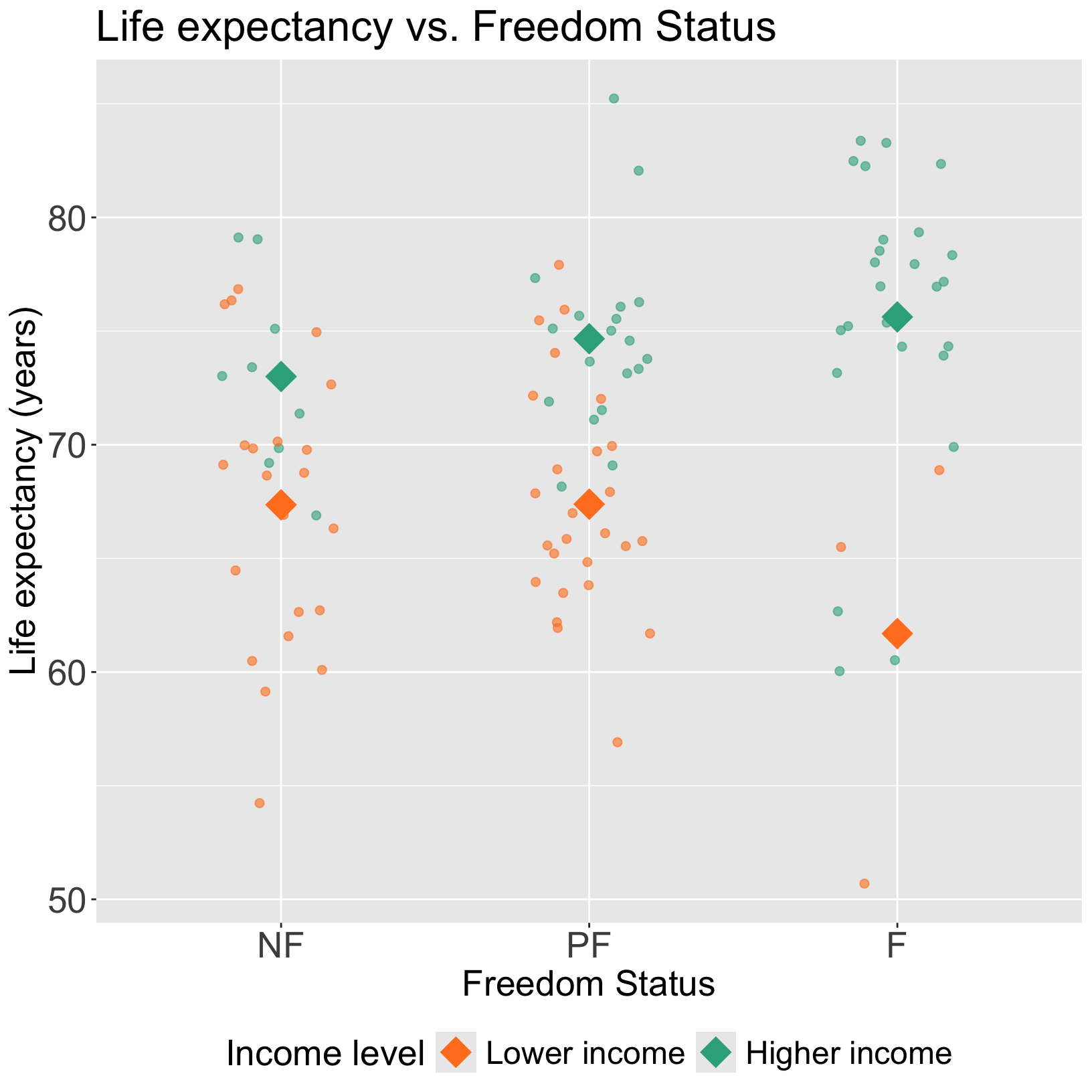
Let’s take a look back at the plot
For lower income countries: \(I(\text{high income}) =0\)
\[ \begin{aligned} \widehat{LE} = & \widehat\beta_0 + \widehat\beta_2 I(\text{FS} = \text{PF}) + \widehat\beta_3 I(\text{FS} = \text{F}) \\ \end{aligned}\]
For higher income countries: \(I(\text{high income}) =1\)
\[ \begin{aligned} \widehat{LE} = & \big(\widehat\beta_0 + \widehat\beta_1 \big) + \big(\widehat\beta_2 + \widehat\beta_4 \big) I(\text{FS} = \text{PF}) + \\ & \big(\widehat\beta_3 + \widehat\beta_5 \big) I(\text{FS} = \text{F}) \\ \end{aligned}\]
Interpretation for interaction between two categorical variables
\[ \begin{aligned} \widehat{LE} = &\widehat\beta_0 + \widehat\beta_1 \cdot 1 + \widehat\beta_2 I(\text{FS} = \text{PF}) + \widehat\beta_3 I(\text{FS} = \text{F}) + \\ & \widehat\beta_4 \cdot 1 \cdot I(\text{FS} = \text{PF}) + \widehat\beta_5 \cdot 1 \cdot I(\text{FS} = \text{F})\\ \widehat{LE} = & \bigg[\widehat\beta_0 + \widehat\beta_1 \cdot I(\text{high income})\bigg] + \bigg[\widehat\beta_2 + \widehat\beta_4 \cdot I(\text{high income})\bigg] I(\text{FS} = \text{PF}) + \\ & \bigg[\widehat\beta_3 + \widehat\beta_5 \cdot I(\text{high income})\bigg] I(\text{FS} = \text{F}) \\ \end{aligned}\]
- Interpretation:
- \(\widehat\beta_1\) = mean change in life expectancy comparing high income to low income countries, for countries/territories that are not free
- \(\widehat\beta_4\) = mean change in life expectancy comparing high income to low income countries, for countries/territories that are partly free
- \(\widehat\beta_5\) = mean change in life expectancy comparing high income to low income countries, for countries/territories that are free
Test interaction between two categorical variables (1/2)
- We run an F-test for a group of coefficients (\(\beta_4\), \(\beta_5\)) in the below model (see lesson 9)
\[\begin{aligned}LE = &\beta_0 + \beta_1 I(\text{high income}) + \beta_2 I(\text{FS} = \text{PF}) + \beta_3 I(\text{FS} = \text{F}) + \\ & \beta_4 \cdot I(\text{high income}) \cdot I(\text{FS} = \text{PF}) + \beta_5 \cdot I(\text{high income}) \cdot I(\text{FS} = \text{F}) + \epsilon \end{aligned}\]
Null \(H_0\)
\(\beta_4= \beta_5 =0\)
Alternative \(H_1\)
\(\beta_4\neq0\) and/or \(\beta_5\neq0\)
Null / Smaller / Reduced model
\[\begin{aligned}LE = &\beta_0 + \beta_1 I(\text{high income}) + \\ &\beta_2 I(\text{FS} = \text{PF}) + \beta_3 I(\text{FS} = \text{F}) + \\ & \epsilon \end{aligned}\]
Alternative / Larger / Full model
\[\begin{aligned}LE = &\beta_0 + \beta_1 I(\text{high income}) + \beta_2 I(\text{FS} = \text{PF}) + \\ & \beta_3 I(\text{FS} = \text{F}) + \beta_4 \cdot I(\text{high income}) \cdot I(\text{FS} = \text{PF}) + \\ & \beta_5 \cdot I(\text{high income}) \cdot I(\text{FS} = \text{F}) + \epsilon \end{aligned}\]
Test interaction between two categorical variables (2/2)
- Fit the reduced and full model
Display the ANOVA table with F-statistic and p-value
| term | df.residual | rss | df | sumsq | statistic | p.value |
|---|---|---|---|---|---|---|
| life_exp ~ income_level_2 + freedom_status | 101.000 | 3,160.771 | NA | NA | NA | NA |
| life_exp ~ income_level_2 * freedom_status | 99.000 | 3,027.855 | 2.000 | 132.915 | 2.173 | 0.119 |
- Conclusion: There is not a significant interaction between freedom status and income level (p = 0.119).
Learning Objectives
Last time:
- Define confounders and effect modifiers, and how they interact with the main relationship we model.
- Interpret the interaction component of a model with a binary categorical covariate and continuous covariate, and how the main variable’s effect changes.
- Interpret the interaction component of a model with a multi-level categorical covariate and continuous covariate, and how the main variable’s effect changes.
This time:
- Interpret the interaction component of a model with two categorical covariates, and how the main variable’s effect changes.
- Interpret the interaction component of a model with two continuous covariates, and how the main variable’s effect changes.
- Report results for a best-fit line (with confidence intervals) at different levels of an effect measure modifier
Do we think vaccination rate is an effect modifier for cell phones?
We can start by visualizing the relationship between life expectancy and cell phones by vaccination rate
Questions of interest: Does the effect of cell phones on life expectancy differ depending on vaccination rate?
- This is the same as: Is vaccination rate is an effect modifier for cell phones? Is vaccination rate an effect modifier of the association between life expectancy and cell phones?
Let’s run an interaction model to see!
Model with interaction between two continuous variables
Model we are fitting:
\[ LE = \beta_0 + \beta_1 CP^c + \beta_2 VR^c + \beta_3 CP^c \cdot VR^c + \epsilon\]
- \(LE\) as life expectancy
- \(CP^c\) as the centered around the mean number of cell phones per 100 people (continuous variable)
- \(VR^c\) as the centered around the mean vaccination rate (continuous variable)
In R:
OR
Displaying the regression table and writing fitted regression equation
| term | estimate | std.error | statistic | p.value | conf.low | conf.high |
|---|---|---|---|---|---|---|
| (Intercept) | 70.56972 | 0.61989 | 113.84216 | 0.00000 | 69.34002 | 71.79942 |
| CP_c | 0.07666 | 0.01832 | 4.18404 | 0.00006 | 0.04032 | 0.11301 |
| VR_c | 0.23765 | 0.08409 | 2.82598 | 0.00568 | 0.07083 | 0.40447 |
| CP_c:VR_c | 0.00308 | 0.00192 | 1.59912 | 0.11292 | −0.00074 | 0.00689 |
\[ \begin{aligned} \widehat{LE} = & \widehat\beta_0 + \widehat\beta_1 CP^c + \widehat\beta_2 VR^c + \widehat\beta_3 CP^c \cdot VR^c \\ \widehat{LE} = & 70.57 + 0.08 \cdot CP^c + 0.24 \cdot VR^c + 0.003 \cdot CP^c \cdot VR^c \end{aligned}\]
Comparing fitted regression lines for various vaccination rates
\[ \begin{aligned} \widehat{LE} = & \widehat\beta_0 + \widehat\beta_1 CP^c + \widehat\beta_2 VR^c + \widehat\beta_3 CP^c \cdot VR^c \\ \widehat{LE} = & 70.57 + 0.08 \cdot CP^c + 0.24 \cdot VR^c + 0.003 \cdot CP^c \cdot VR^c \end{aligned}\]
To identify different lines, we need to pick example vaccination rates:
Vaccination rate of 86.45 %
\[\begin{aligned} \widehat{LE} = & \widehat\beta_0 + \widehat\beta_1 CP^c + \\ & \widehat\beta_2 \cdot (-5) + \\ & \widehat\beta_3 CP^c \cdot (-5) \\ \widehat{LE} = & \big(\widehat\beta_0 - 5 \widehat\beta_2 \big)+ \\ & \big(\widehat\beta_1 - 5 \widehat\beta_3 \big) CP^c \end{aligned}\]
Vaccination rate of 91.45 %
\[\begin{aligned} \widehat{LE} = & \widehat\beta_0 + \widehat\beta_1 CP^c + \\ & \widehat\beta_2 \cdot 0 + \\ & \widehat\beta_3 CP^c \cdot 0 \\ \widehat{LE} = & \big(\widehat\beta_0 \big)+ \\ & \big(\widehat\beta_1 \big) CP^c \end{aligned}\]
Vaccination rate of 96.45 %
\[\begin{aligned} \widehat{LE} = & \widehat\beta_0 + \widehat\beta_1 CP^c + \\ & \widehat\beta_2 \cdot 5 + \\ & \widehat\beta_3 CP^c \cdot 5 \\ \widehat{LE} = & \big(\widehat\beta_0 + 5 \widehat\beta_2 \big)+ \\ & \big(\widehat\beta_1 + 5 \widehat\beta_3 \big) CP^c \end{aligned}\]
Poll Everywhere Question??
Interpretation for interaction between two continuous variables
\[ \begin{aligned} \widehat{LE} = & \widehat\beta_0 + \widehat\beta_1 CP^c + \widehat\beta_2 VR^c + \widehat\beta_3 CP^c \cdot VR^c \\ \widehat{LE} = & \bigg[\widehat\beta_0 + \widehat\beta_2 \cdot VR^c \bigg] + \underbrace{\bigg[\widehat\beta_1 + \widehat\beta_3 \cdot VR^c \bigg]}_\text{CP's effect} CP \\ \end{aligned}\]
Interpretation:
- \(\beta_3\) = mean change in cell phones’s effect, for every 1 % increase in vaccination rate
In summary, the interaction term can be interpreted as “difference in adjusted effect of number of cell phones for every 1 % increase in vaccination rate”
It will be helpful to test the interaction to round out this interpretation!!
Test interaction between two continuous variables (1/2)
- We run an F-test for a single coefficients (\(\beta_3\)) in the below model (see lesson 9)
\[ LE = \beta_0 + \beta_1 CP^c + \beta_2 VR^c + \beta_3 CP^c \cdot VR^c + \epsilon\]
Null \(H_0\)
\[\beta_3=0\]
Alternative \(H_1\)
\[\beta_3\neq0\]
Null / Smaller / Reduced model
\[ LE = \beta_0 + \beta_1 CP^c + \beta_2 VR^c + \epsilon\]
Alternative / Larger / Full model
\[\begin{aligned} LE = & \beta_0 + \beta_1 CP^c + \beta_2 VR^c + \\ & \beta_3 CP^c \cdot VR^c + \epsilon \end{aligned}\]
Test interaction between two continuous variables (2/2)
- Fit the reduced and full model
Display the ANOVA table with F-statistic and p-value
| term | df.residual | rss | df | sumsq | statistic | p.value |
|---|---|---|---|---|---|---|
| life_exp ~ CP_c + VR_c | 102.000 | 3,480.371 | NA | NA | NA | NA |
| life_exp ~ CP_c + VR_c + CP_c * VR_c | 101.000 | 3,394.429 | 1.000 | 85.942 | 2.557 | 0.113 |
- Conclusion: There is not a significant interaction between cell phones and vaccination rate (p = 0.113). Vaccination rate is not an effect modifier of the association between cell phones and life expectancy.
Learning Objective
Last time:
- Define confounders and effect modifiers, and how they interact with the main relationship we model.
- Interpret the interaction component of a model with a binary categorical covariate and continuous covariate, and how the main variable’s effect changes.
- Interpret the interaction component of a model with a multi-level categorical covariate and continuous covariate, and how the main variable’s effect changes.
This time:
- Interpret the interaction component of a model with two categorical covariates, and how the main variable’s effect changes.
- Interpret the interaction component of a model with two continuous covariates, and how the main variable’s effect changes.
- Report results for a best-fit line (with confidence intervals) at different levels of an effect measure modifier
How to find the confidence interval for each slope?
- In the example with VR and CP, we showed:
Best-fit line for vaccination rate of 96.45 %
\[\begin{aligned} \widehat{LE} = & \big(\widehat\beta_0 + 5 \widehat\beta_2 \big)+ \big(\widehat\beta_1 + 5 \widehat\beta_3 \big) CP^c \end{aligned}\]
Often, we want to report the estimate of the combined coefficients: \(\widehat\beta_1 + 5 \widehat\beta_3\)
- This allows us to make a statement like: “At a vaccination rate of 96.45%, mean life expectancy increases \(\big(\widehat\beta_1 + 5 \widehat\beta_3 \big)\) years for every one additional cell phone per 100 people (95% CI: __, __).”
We can calculate \(\widehat\beta_1 + 5 \widehat\beta_3\) by using the values of the estimated coefficients
BUT we always want to have a 95% confidence interval when we report this combined estimate!!
Getting a 95% confidence interval requires linear combinations!
- If we want a confidence interval for \(\widehat\beta_1 + 5 \widehat\beta_3\), then we would use the formula:
\[\bigg(\widehat\beta_1 + 5 \widehat\beta_3 \bigg) \pm t^* \times SE_{(\beta_1 + 5 \beta_3)}\]
The hard part is figuring out what \(SE_{(\beta_1 + 5 \beta_3)}\) (or \(\text{Var}(\beta_1 + 5 \beta_3)\)) equals
We need to go back to variance of linear combinations (BSTA 511/611, EPI 525): \[\text{Var}(aX + bY) = a^2\text{Var}(X) + b^2\text{Var}(Y) + 2ab\text{Cov}(X, Y)\] or \[\text{Var}(aX - bY) = a^2\text{Var}(X) + b^2\text{Var}(Y) - 2ab\text{Cov}(X, Y)\]
Calculating \(SE_{(\beta_1 + 5 \beta_3)}\) “by hand” (REFERENCE)
- A helpful function that returns the variance-covariance matric of all the coefficients in model
m_int_vr:
\[ \begin{aligned} \text{Var}(\beta_1) & = 3.35733\times 10^{-4} \\ \text{Var}(\beta_3) & = 0.0070718 \\ \text{Cov}(\beta_1, \beta_3) & = -5.35492\times 10^{-4} \\ \end{aligned}\]
\[ \begin{aligned} \text{Var}(\beta_1 + 5 \beta_3) & = \text{Var}(\beta_1) + 5 ^2 \text{Var}(\beta_3) + 2 \cdot 5 \cdot \text{Cov}(\beta_1, \beta_3) \\ \text{Var}(\beta_1 + 5 \beta_3) & = 3.35733\times 10^{-4} + 5^2 \ \times 3.7\times 10^{-6} + 2 \cdot 5 \cdot 1.872\times 10^{-6} \\ \text{Var}(\beta_1 + 5 \beta_3) & = 4.46967\times 10^{-4} \\ SE_{(\beta_1 + 5 \beta_3)} & = \sqrt{4.46967\times 10^{-4}} \\ SE_{(\beta_1 + 5 \beta_3)} & = 0.0211416 \end{aligned}\]
We can use R and estimable() to find the estimate and CI
For \(\widehat\beta_1 + 5 \widehat\beta_3\):
            Estimate Std. Error t value  DF     Pr(>|t|)   Lower.CI Upper.CI
(0 1 0 5) 0.09204476 0.02114159 4.35373 101 3.213735e-05 0.05010553 0.133984
Our conclusion: At a vaccination rate of 96.45 %, mean life expectancy increases 0.092 years for every one additional cell phone per 100 people (95% CI: 0.05, 0.134).
Another example: income (binary) and CP (1/2)
\[ \begin{aligned} \widehat{LE} = & \widehat\beta_0 + \widehat\beta_1 CP^c + \widehat\beta_2 I(\text{high income}) + \widehat\beta_3 CP^c \cdot I(\text{high income}) \\ \widehat{LE} = & 68.408 + 0.076 \cdot CP^c + 6.247 \cdot I(\text{high income}) -0.066 \cdot CP^c \cdot I(\text{high income}) \end{aligned}\]
For lower income countries: \(I(\text{high income}) =0\)
\[ \begin{aligned} \widehat{LE} = & \widehat\beta_0 + \widehat\beta_1 CP\\ \widehat{LE} = & 68.41 + 0.076 \cdot CP \end{aligned}\]
For higher income countries: \(I(\text{high income}) =1\)
\[ \begin{aligned} \widehat{LE} = & (\widehat\beta_0 +\widehat\beta_2) + (\widehat\beta_1 +\widehat\beta_3) CP \\ \widehat{LE} = & (68.41 + 6.247) + (0.076 -0.066) \cdot CP \\ \widehat{LE} = & 74.65 + 0.01 \cdot CP \end{aligned}\]
Another example: income (binary) and CP (2/2)
[1] "(Intercept)"                      "CP_c"
[3] "income_level_2Higher income" "CP_c:income_level_2Higher income" Estimate Std. Error t value DF Pr(>|t|) Lower.CI Upper.CI
(0 1 0 1) 0.01001064 0.02723878 0.3675143 101 0.7140044 -0.04402377 0.06404504
Our conclusion: For countries with high income, mean life expectancy increases 0.01 years for every one additional cell phone per 100 people (95% CI: -0.044, 0.064).
If our example had an effect measure modifier
None of our examples had a significant interaction, so it’s hard to demonstrate exactly how we would report this
Let’s say, just for example, that income had a significant interaction with CP
- How would we report this to an audience??
Here’s how to report on an interaction/EMM:
- We found that a country’s income status (high or low) is a significant effect measure modifier on number of cell phones (include p-value for interaction test here). For countries with high income, mean life expectancy increases 0.01 years for every additional cell phone per 100 people (95% CI: -0.044, 0.064). For countries with low income, mean life expectancy increases 6.247 years for every additional cell phone per 100 people (95% CI: 3.825, 8.668).
Lesson 12: Interactions 2