Lesson 2: Data and File Management

Adapted from parts of Mine Çetinkaya-Rundel’s tidyverse course

Nicky Wakim

2025-01-08

What we will cover

1. Introduction to tidyverse
2. ggplot2 revisited
3. Functions for data management
4. Functions for data summarization
5. Folder organization
6. here package and importing data

 

• Not covered: basic Quarto set up. Please see R recordings in OneDrive and my EPI 525 site for videos and slides.

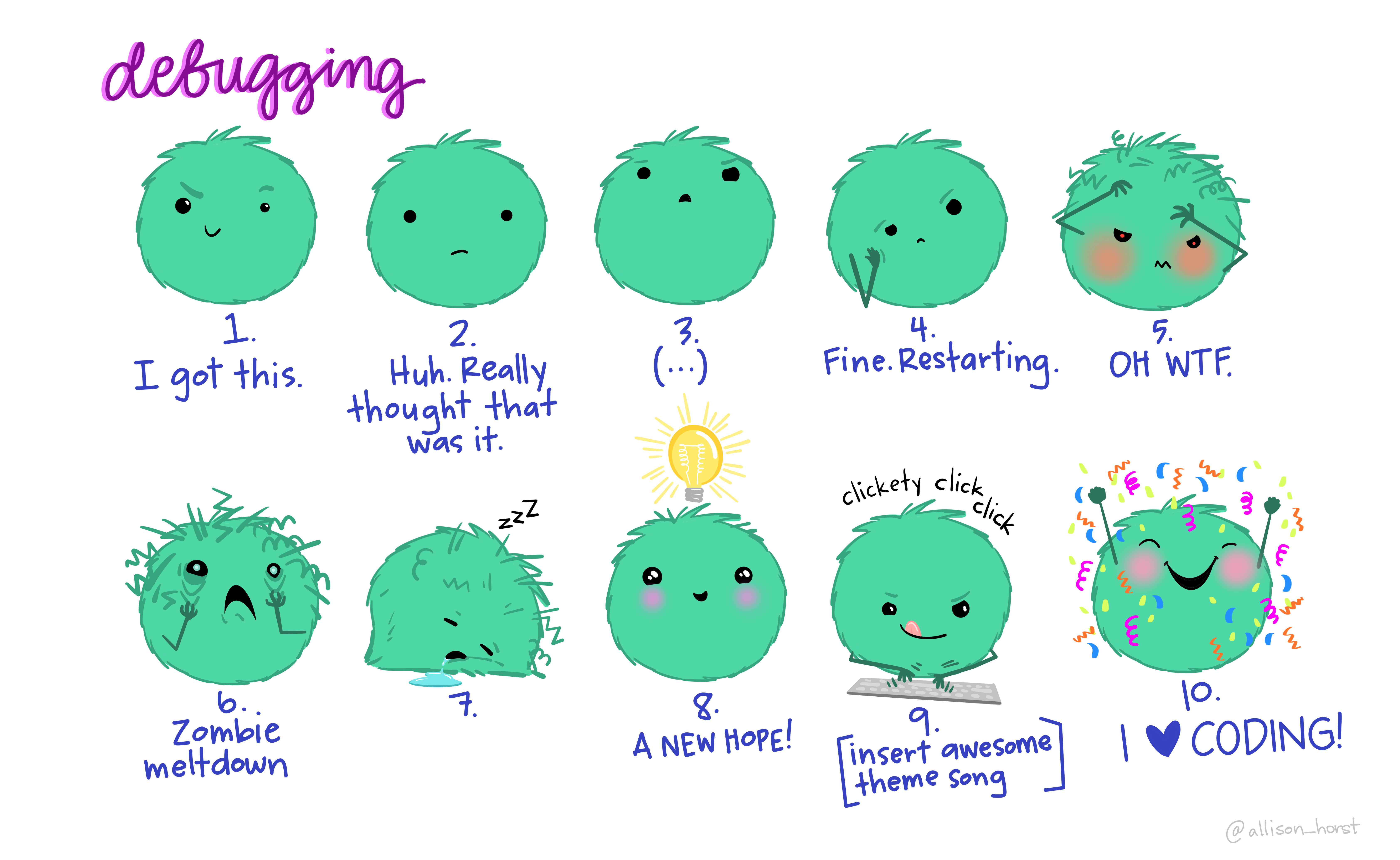
Artwork by @allison_horst

Introduction to the tidyverse

What is the tidyverse?

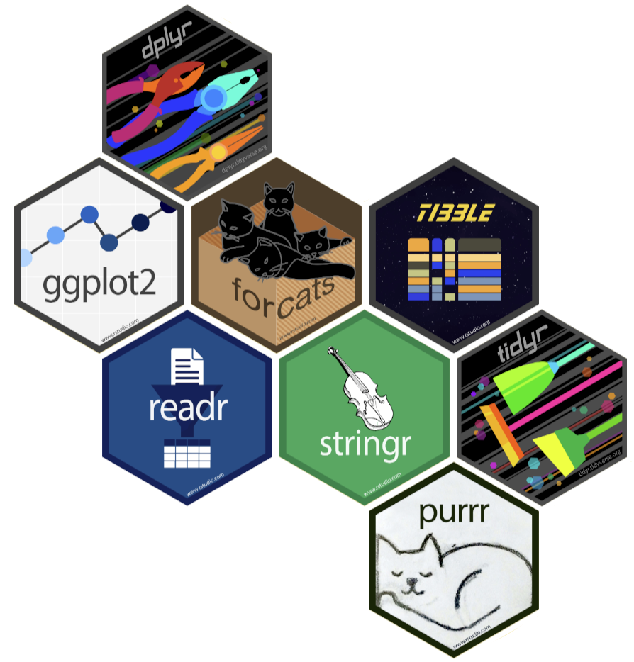
The tidyverse is a collection of R packages designed for data science. All packages share an underlying design philosophy, grammar, and data structures.

• ggplot2 - data visualisation
• dplyr - data manipulation
• tidyr - tidy data
• readr - read rectangular data
• purrr - functional programming
• tibble - modern data frames
• stringr - string manipulation
• forcats - factors
• and many more …

Tidy data¹

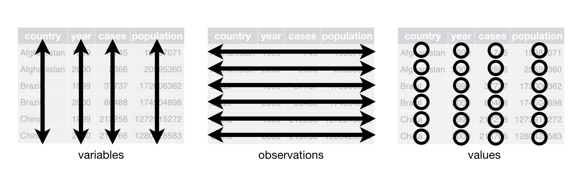
1. Each variable must have its own column.

2. Each observation must have its own row.

3. Each value must have its own cell.

1. Source: R for Data Science. Grolemund and Wickham.

Pipe operator (magrittr)

• The pipe operator (%>%) allows us to step through sequential functions in the same way we follow if-then statements or steps from instructions

 

I want to find my keys, then start my car, then drive to work, then park my car.

 

Nested

park(drive(start_car(find("keys")), 
           to = "work"))

Piped

find("keys") %>%
  start_car() %>%
  drive(to = "work") %>%
  park()

Recoding a binary variable with pipe operator

 

Let’s say I want a variable transmission to show the category names that are assigned to numeric values in the code. I want 0 to be coded as automatic and 1 to be coded as manual.

 

Base R:

mtcars$transmission <-
  ifelse(
    mtcars$am == 0,
    "automatic",
    "manual"
  )

Tidyverse:

mtcars <- mtcars %>%
  mutate(
    transmission = case_when(
      am == 0 ~ "automatic",
      am == 1 ~ "manual"
    )
  )

 

mutate() creates new columns that are functions of existing variables

Recoding a multi-level variable

 

Let’s say I want a variable gear to show the category names that are assigned to numeric values in the code. I want 3 to be coded as gear three, 4 to be coded as gear four, 5 to be coded as gear five.

 

Base R:

mtcars$gear_char <-
  ifelse(
    mtcars$gear == 3,
    "three",
    ifelse(
      mtcars$gear == 4,
      "four",
      "five"
    )
  )

Tidyverse:

mtcars <- mtcars %>%
  mutate(
    gear_char = case_when(
      gear == 3 ~ "three",
      gear == 4 ~ "four",
      gear == 5 ~ "five"
    )
  )

ggplot2 revisited

ggplot2 in tidyverse

• We talked about this in our review notes

  • I want to revisit it: always helps to have more examples!
  • This example is closer to the multivariable work we’ll do in this class!

 

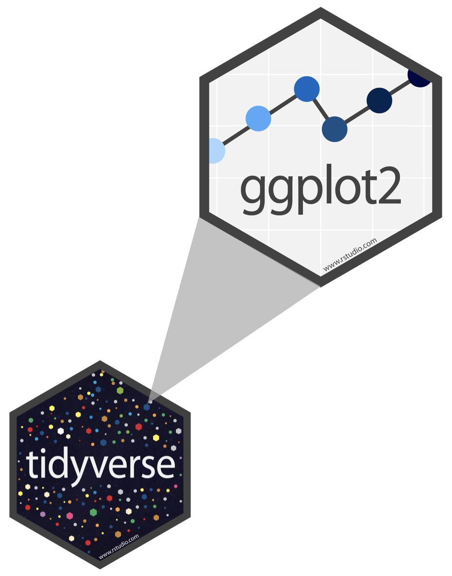
• ggplot2 is tidyverse’s data visualization package

 

• The gg in “ggplot2” stands for Grammar of Graphics

 

• It is inspired by the book Grammar of Graphics by Leland Wilkinson

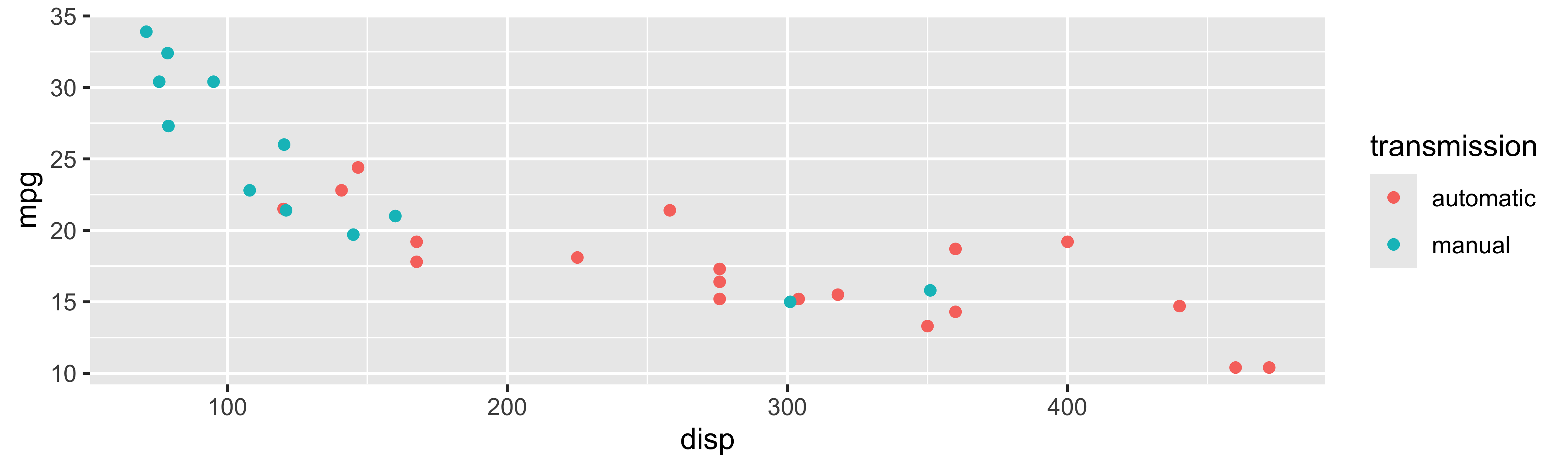
Tidyverse: Visualizing multiple variables

 

ggplot(
  mtcars,
  aes(x = disp, y = mpg, color = transmission)) +
  geom_point()

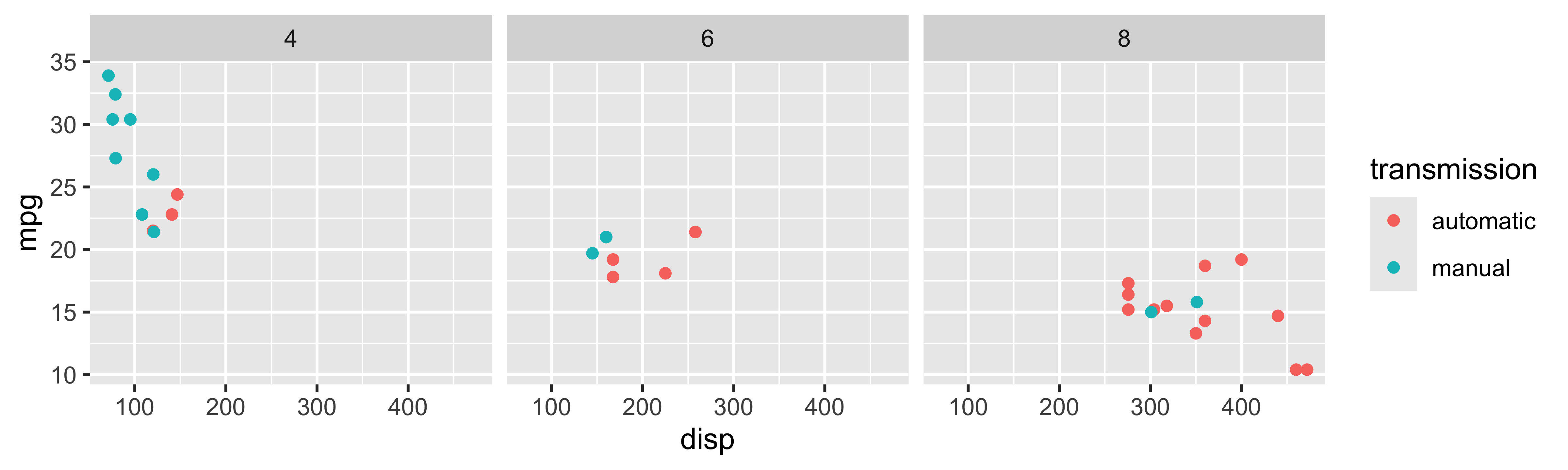
Tidyverse: Visualizing even more variables

ggplot(
  mtcars,
  aes(x = disp, y = mpg, color = transmission)) +
  geom_point() +
  facet_wrap(~ cyl)

Base R: Visualizing even more variables

mtcars$trans_color <- ifelse(mtcars$transmission == "automatic", "green", "blue")
mtcars_cyl4 = mtcars[mtcars$cyl == 4, ]
mtcars_cyl6 = mtcars[mtcars$cyl == 6, ]
mtcars_cyl8 = mtcars[mtcars$cyl == 8, ]
par(mfrow = c(1, 3), mar = c(2.5, 2.5, 2, 0), mgp = c(1.5, 0.5, 0))
plot(mpg ~ disp, data = mtcars_cyl4, col = trans_color, main = "Cyl 4")
plot(mpg ~ disp, data = mtcars_cyl6, col = trans_color, main = "Cyl 6")
plot(mpg ~ disp, data = mtcars_cyl8, col = trans_color, main = "Cyl 8")
legend("topright", legend = c("automatic", "manual"), pch = 1, col = c("green", "blue"))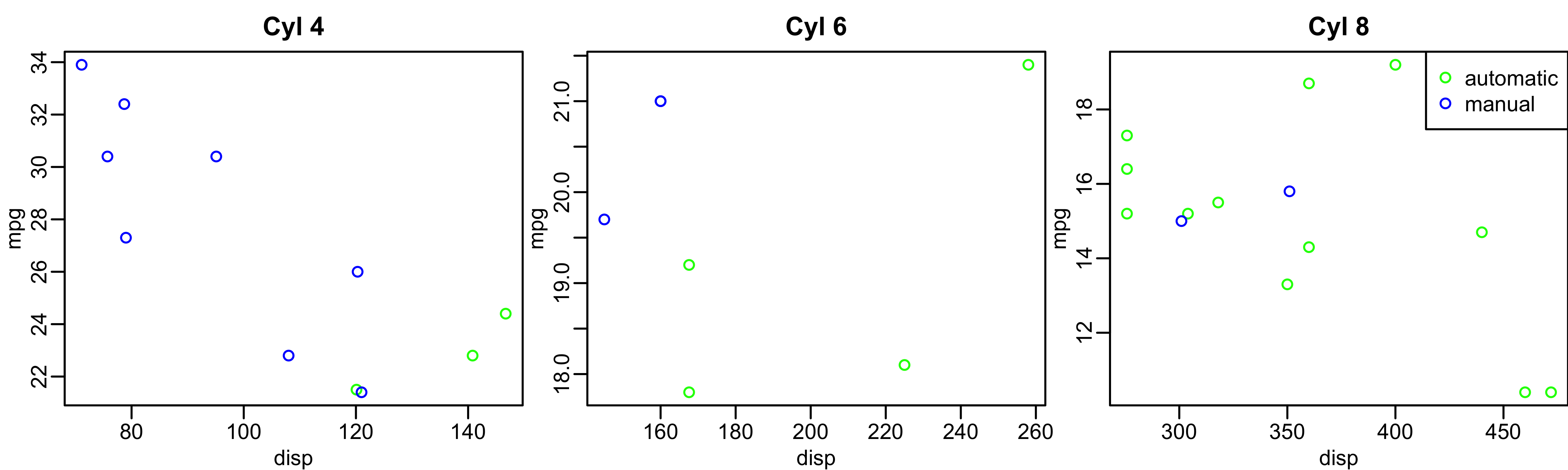

Functions for data management

Important functions for data management

 

Data manipulation

• pivot_longer() and pivot_wider() (not covered today)

• rename()

• mutate()

• filter()

• select()

Summarizing data

• tbl_summary()
• group_by()
• summarize()
• across()

Let’s look back at the dds.discr dataset that I briefly used last class

   

• We will load the data (This is a special case! dds.discr is a built-in R dataset)

data("dds.discr")

• Now, let’s take a glimpse at the dataset:

glimpse(dds.discr)

Rows: 1,000
Columns: 6
$ id           <int> 10210, 10409, 10486, 10538, 10568, 10690, 10711, 10778, 1…
$ age.cohort   <fct> 13-17, 22-50, 0-5, 18-21, 13-17, 13-17, 13-17, 13-17, 13-…
$ age          <int> 17, 37, 3, 19, 13, 15, 13, 17, 14, 13, 13, 14, 15, 17, 20…
$ gender       <fct> Female, Male, Male, Female, Male, Female, Female, Male, F…
$ expenditures <int> 2113, 41924, 1454, 6400, 4412, 4566, 3915, 3873, 5021, 28…
$ ethnicity    <fct> White not Hispanic, White not Hispanic, Hispanic, Hispani…

rename(): one of the first things I usually do

• I notice that two variables have values that don’t necessarily match the variable name

  • Female and male are not genders

  • “White not Hispanic” combines race and ethnicity into one category

I want to rename gender to SAB (sex assigned at birth) and rename ethnicity to R_E (race and ethnicity)

 

dds.discr1 = dds.discr %>% 
  rename(SAB = gender, 
         R_E = ethnicity)

glimpse(dds.discr1)

Rows: 1,000
Columns: 6
$ id           <int> 10210, 10409, 10486, 10538, 10568, 10690, 10711, 10778, 1…
$ age.cohort   <fct> 13-17, 22-50, 0-5, 18-21, 13-17, 13-17, 13-17, 13-17, 13-…
$ age          <int> 17, 37, 3, 19, 13, 15, 13, 17, 14, 13, 13, 14, 15, 17, 20…
$ SAB          <fct> Female, Male, Male, Female, Male, Female, Female, Male, F…
$ expenditures <int> 2113, 41924, 1454, 6400, 4412, 4566, 3915, 3873, 5021, 28…
$ R_E          <fct> White not Hispanic, White not Hispanic, Hispanic, Hispani…

mutate(): constructing new variables from what you have

• We’ve seen a couple examples for mutate() so far (mostly because its used so often!)

• We haven’t seen an example where we make a new variable from two variables

I want to make a variable that is the ratio of expenditures over age

 

dds.discr2 = dds.discr1 %>%
  mutate(exp_to_age = expenditures/age)

glimpse(dds.discr2)

Rows: 1,000
Columns: 7
$ id           <int> 10210, 10409, 10486, 10538, 10568, 10690, 10711, 10778, 1…
$ age.cohort   <fct> 13-17, 22-50, 0-5, 18-21, 13-17, 13-17, 13-17, 13-17, 13-…
$ age          <int> 17, 37, 3, 19, 13, 15, 13, 17, 14, 13, 13, 14, 15, 17, 20…
$ SAB          <fct> Female, Male, Male, Female, Male, Female, Female, Male, F…
$ expenditures <int> 2113, 41924, 1454, 6400, 4412, 4566, 3915, 3873, 5021, 28…
$ R_E          <fct> White not Hispanic, White not Hispanic, Hispanic, Hispani…
$ exp_to_age   <dbl> 124.2941, 1133.0811, 484.6667, 336.8421, 339.3846, 304.40…

mutate(): other examples

dds.discr3 = dds.discr1 %>%
  mutate(expend_20perc = expenditures * 0.2, 
         expend_sq = expenditures^2, 
         expend_over_5000 = case_when(
           expenditures > 5000 ~ "Yes", 
           expenditures <= 5000 ~ "No"
         ), 
         expend_log = log(expenditures)
  )
glimpse(dds.discr3)

Rows: 1,000
Columns: 10
$ id               <int> 10210, 10409, 10486, 10538, 10568, 10690, 10711, 1077…
$ age.cohort       <fct> 13-17, 22-50, 0-5, 18-21, 13-17, 13-17, 13-17, 13-17,…
$ age              <int> 17, 37, 3, 19, 13, 15, 13, 17, 14, 13, 13, 14, 15, 17…
$ SAB              <fct> Female, Male, Male, Female, Male, Female, Female, Mal…
$ expenditures     <int> 2113, 41924, 1454, 6400, 4412, 4566, 3915, 3873, 5021…
$ R_E              <fct> White not Hispanic, White not Hispanic, Hispanic, His…
$ expend_20perc    <dbl> 422.6, 8384.8, 290.8, 1280.0, 882.4, 913.2, 783.0, 77…
$ expend_sq        <dbl> 4464769, 1757621776, 2114116, 40960000, 19465744, 208…
$ expend_over_5000 <chr> "No", "Yes", "No", "Yes", "No", "No", "No", "No", "Ye…
$ expend_log       <dbl> 7.655864, 10.643614, 7.282074, 8.764053, 8.392083, 8.…

filter(): keep rows that match a condition

• What if I want to subset the data frame? (keep certain rows of observations)

I want to look at the data for people who between 50 and 60 years old

 

dds.discr3 = dds.discr2 %>%
  filter(age >= 50 & age <= 60)

glimpse(dds.discr3)

Rows: 23
Columns: 7
$ id           <int> 15970, 19412, 29506, 31658, 36123, 39287, 39672, 43455, 4…
$ age.cohort   <fct> 51+, 51+, 51+, 51+, 51+, 51+, 51+, 51+, 51+, 51+, 51+, 51…
$ age          <int> 51, 60, 56, 60, 59, 59, 54, 57, 52, 57, 55, 52, 59, 54, 5…
$ SAB          <fct> Female, Female, Female, Female, Male, Female, Female, Mal…
$ expenditures <int> 54267, 57702, 48215, 46873, 42739, 44734, 52833, 48363, 5…
$ R_E          <fct> White not Hispanic, White not Hispanic, White not Hispani…
$ exp_to_age   <dbl> 1064.0588, 961.7000, 860.9821, 781.2167, 724.3898, 758.20…

select(): keep or drop columns using their names and types

• What if I want to remove or keep certain variables?

I want to only have age and expenditure in my data frame

 

dds.discr4 = dds.discr2 %>%
  select(age, expenditures)

glimpse(dds.discr4)

Rows: 1,000
Columns: 2
$ age          <int> 17, 37, 3, 19, 13, 15, 13, 17, 14, 13, 13, 14, 15, 17, 20…
$ expenditures <int> 2113, 41924, 1454, 6400, 4412, 4566, 3915, 3873, 5021, 28…

Summarizing Data

tbl_summary() : table summary (1/2)

• What if I want one of those fancy summary tables that are at the top of most research articles? (lovingly called “Table 1”)

library(gtsummary)
tbl_summary(dds.discr2)

Characteristic	N = 1,0001
id	55,385 (31,759, 76,205)
age.cohort
0-5	82 (8.2%)
6-12	175 (18%)
13-17	212 (21%)
18-21	199 (20%)
22-50	226 (23%)
51+	106 (11%)
age	18 (12, 26)
SAB
Female	503 (50%)
Male	497 (50%)
expenditures	7,026 (2,898, 37,718)
R_E
American Indian	4 (0.4%)
Asian	129 (13%)
Black	59 (5.9%)
Hispanic	376 (38%)
Multi Race	26 (2.6%)
Native Hawaiian	3 (0.3%)
Other	2 (0.2%)
White not Hispanic	401 (40%)
exp_to_age	462 (273, 938)
1 Median (Q1, Q3); n (%)

tbl_summary() : table summary (2/2)

• Let’s make this more presentable

 

dds.discr2 %>%
  select(-id, -age.cohort, -exp_to_age) %>%
  tbl_summary(label = c(age ~ "Age", 
                        R_E ~ "Race/Ethnicity", 
                        SAB ~ "Sex Assigned at Birth", 
                        expenditures ~ "Expenditures") ,
              statistic = list(all_continuous() ~ "{mean} ({sd})"))

Characteristic	N = 1,0001
Age	23 (18)
Sex Assigned at Birth
Female	503 (50%)
Male	497 (50%)
Expenditures	18,066 (19,543)
Race/Ethnicity
American Indian	4 (0.4%)
Asian	129 (13%)
Black	59 (5.9%)
Hispanic	376 (38%)
Multi Race	26 (2.6%)
Native Hawaiian	3 (0.3%)
Other	2 (0.2%)
White not Hispanic	401 (40%)
1 Mean (SD); n (%)

group_by(): group by one or more variables

• What if I want to quickly look at group differences?
• It will not change how the data look, but changes the actions of following functions

I want to group my data by sex assigned at birth.

 

dds.discr5 = dds.discr2 %>%
  group_by(SAB)
glimpse(dds.discr5)

Rows: 1,000
Columns: 7
Groups: SAB [2]
$ id           <int> 10210, 10409, 10486, 10538, 10568, 10690, 10711, 10778, 1…
$ age.cohort   <fct> 13-17, 22-50, 0-5, 18-21, 13-17, 13-17, 13-17, 13-17, 13-…
$ age          <int> 17, 37, 3, 19, 13, 15, 13, 17, 14, 13, 13, 14, 15, 17, 20…
$ SAB          <fct> Female, Male, Male, Female, Male, Female, Female, Male, F…
$ expenditures <int> 2113, 41924, 1454, 6400, 4412, 4566, 3915, 3873, 5021, 28…
$ R_E          <fct> White not Hispanic, White not Hispanic, Hispanic, Hispani…
$ exp_to_age   <dbl> 124.2941, 1133.0811, 484.6667, 336.8421, 339.3846, 304.40…

• Let’s see how the groups change something like the summarize() function in the next slide

summarize(): summarize your data or grouped data into one row

• What if I want to calculate specific descriptive statistics for my variables?
• This function is often best used with group_by()
• If only presenting the summaries, functions like tbl_summary() is better
• summarize() creates a new data frame, which means you can plot and manipulate the summarized data

 

Over whole sample:

dds.discr2 %>% 
  summarize(
    ave = mean(expenditures),
    SD = sd(expenditures),
    med = median(expenditures))

# A tibble: 1 × 3
     ave     SD   med
   <dbl>  <dbl> <dbl>
1 18066. 19543.  7026

Grouped by sex assigned at birth:

dds.discr2 %>% 
  group_by(SAB) %>% 
  summarize(
    ave = mean(expenditures),
    SD = sd(expenditures),
    med = median(expenditures))

# A tibble: 2 × 4
  SAB       ave     SD   med
  <fct>   <dbl>  <dbl> <int>
1 Female 18130. 20020.  6400
2 Male   18001. 19068.  7219

across(): apply a function across multiple columns

• Like group_by(), this function is often paired with another transformation function

I want all my integer values to have two significant figures.

 

dds.discr6 = dds.discr2 %>%
  mutate(across(where(is.integer), signif, digits = 2))

glimpse(dds.discr6)

Rows: 1,000
Columns: 7
$ id           <dbl> 10000, 10000, 10000, 11000, 11000, 11000, 11000, 11000, 1…
$ age.cohort   <fct> 13-17, 22-50, 0-5, 18-21, 13-17, 13-17, 13-17, 13-17, 13-…
$ age          <dbl> 17, 37, 3, 19, 13, 15, 13, 17, 14, 13, 13, 14, 15, 17, 20…
$ SAB          <fct> Female, Male, Male, Female, Male, Female, Female, Male, F…
$ expenditures <dbl> 2100, 42000, 1500, 6400, 4400, 4600, 3900, 3900, 5000, 29…
$ R_E          <fct> White not Hispanic, White not Hispanic, Hispanic, Hispani…
$ exp_to_age   <dbl> 124.2941, 1133.0811, 484.6667, 336.8421, 339.3846, 304.40…

Folder organization

Folder organization

• Make a folder for our class!

  • I suggest naming it something like BSTA_512_W25 to indicate the class and the term

• Make these folders in your computer (or in OneDrive if you prefer)

  • Only make them in OneDrive if you have a desktop connection

• For a project, I have the following folders

  • Background
  • Code
  • Data_Raw
  • Data_Processed
  • Dissemination
  • Reports
  • Meetings

• For our class, I suggest making one folder for the course with the following folders in it:

  • Data
  • Homework
  • Project (with above subfolders)
  • Lessons
  • And other folders if you want

Aside: folder and file naming

There are a few good practices for naming files and folders for easy tracking:

1. Keep the name short and relevant
2. Use leading numbers to help organize sequential items
   • I can show you my lessons folders as an example
3. Use dates in the format “YYYY-MM-DD” so that files are in chronological order
4. You can label different versions if you would like to
5. Use “_” to separate sections of the name
   • I also use this to separate words, but some people say you should use “-” to separate words

Creating project in RStudio

• Way to designate a working directory: basically your home base when working in R

  • We have to tell R exactly where we are in our folders and where to find other things

  • A project makes it easier to tell R where we are

• Basic steps to create a project

  • Go into RStudio

  • Create new project for this class (under File or top right corner)

    • I would chose “Existing Directory” since we have already set up our folders
    • Make the new project in the BSTA_512_W25 folder

• Once we have projects, we can open one and R will automatically know that its location is the start of our working directory

• Only make one project for now!!

The nice thing about R projects

• 5 minute video explaining some of the nice features of R projects

https://rfortherestofus.com/2022/10/rstudio-projects

Reproducibility

• Research data and code can reach the same results regardless of who is running the code

  • This can also refer to future or past you!

 

• We want to set up our work so the entire folder can be moved around and work in its new location

 

• Projects work well in combination with the here package

here package and importing data

here package

Illustration by Allison Horst

here package

• Good source for the here package

  • Just substitute .Rmd with .qmd

• Basically, a .qmd file and .R file work differently

  • We haven’t worked much with .R files

• For .qmd files, the automatic directory is the folder it is in

  • But we want it to be the main project folder

• here can help with that

 

• Very important for reproducibility!!

Using here package

• Within your console, type here() and enter

  • Try this with getwd() as well

library(here)
here()

[1] "/Users/wakim/Library/CloudStorage/OneDrive-OregonHealth&ScienceUniversity/Teaching/Classes/W25_BSTA_512_612/BSTA_512_W25_site"

getwd()

[1] "/Users/wakim/Library/CloudStorage/OneDrive-OregonHealth&ScienceUniversity/Teaching/Classes/W25_BSTA_512_612/BSTA_512_W25_site"

 

• here can be used whenever we need to access a file path in R code
  • Importing data
  • Saving output
  • Accessing files

Importing data

Using here() to load data

• The here() function will start at the working directory (where your .Rproj file is) and let you write out a file path for anything

• To load the dataset in our .qmd file, we will use:

library(readxl)
data = read_excel(here("./data/BodyTemperatures.xlsx"))
data = read_excel(here("data", "BodyTemperatures.xlsx"))

Common functions to load data

Function	Data file type	Package needed
read_excel()	.xls, .xlsx	readxl
read.csv()	.csv	Built in
load()	.Rdata	Built in
read_sas()	.sas7bdat	haven

Resources

dplyr resources

• More dpylr functions to reference!

Additional details and examples are available in the vignettes:

• column-wise operations vignette

• row-wise operations vignette

 

and the dplyr 1.0.0 release blog posts:

• working across columns
• working within rows

R programming class at OHSU!

You can check out Dr. Jessica Minnier’s R class page if you want more notes, videos, etc.

The larger tidy ecosystem

Just to name a few…

• janitor

• kableExtra

• patchwork

• gghighlight

• tidybayes

Credit to Mine Çetinkaya-Rundel

• These notes were built from Mine’s notes

  • Most pages and code were left as she made them

  • I changed a few things to match our class

• Please see her Github repository for the original notes