Lesson 9: Introduction to Multiple Linear Regression (MLR)
2025-02-05
Learning Objectives
- Understand the population multiple linear regression model through equations and visuals.
- Fit MLR model (in
R) and understand the difference between fitted regression plane and regression lines. - Interpret MLR (population) coefficient estimates with additional variable in model
- Based off of previous SLR work, understand how the population MLR is estimated.
Reminder of what we learned in the context of SLR
SLR helped us establish the foundation for a lot of regression
- But we do not usually use SLR in analysis
What did we learn in SLR??
Model Fitting
- Ordinary least squares (OLS)
lm()function in R
Model Use
- Inference for variance of residuals
- Hypothesis testing for coefficients
- Interpreting population coefficient estimates
- Calculated the expected mean for specific \(X\) values
- Interpreted coefficient of determination
Model Evaluation/Diagnostics
- LINE Assumptions
- Influential points
- Data Transformations
Let’s map that to our regression analysis process

![]()
![]()
Model Selection
Building a model
Selecting variables
Prediction vs interpretation
Comparing potential models
Model Fitting
Find best fit line
Using OLS in this class
Parameter estimation
Categorical covariates
Interactions
Model Evaluation
- Evaluation of model fit
- Testing model assumptions
- Residuals
- Transformations
- Influential points
- Multicollinearity
Model Use (Inference)
- Inference for coefficients
- Hypothesis testing for coefficients
- Inference for expected \(Y\) given \(X\)

Learning Objectives
- Understand the population multiple linear regression model through equations and visuals.
- Fit MLR model (in
R) and understand the difference between fitted regression plane and regression lines. - Interpret MLR (population) coefficient estimates with additional variable in model
- Based off of previous SLR work, understand how the population MLR is estimated.
Simple Linear Regression vs. Multiple Linear Regression
Simple Linear Regression
We use one predictor to try to explain the variance of the outcome
\[ Y = \beta_0 + \beta_1 X + \epsilon \]
Multiple Linear Regression
We use multiple predictors to try to explain the variance of the outcome
\[ Y = \beta_0 + \beta_1 X_1 + \beta_2 X_2 + ... + \beta_{k}X_{k}+ \epsilon \]
- Has \(k+1\) total coefficients (including intercept) for \(k\) predictors/covariates
- Sometimes referred to as multivariable linear regression, but never multivariate
- The models have similar “LINE” assumptions and follow the same general diagnostic procedure
Population multiple regression model
\[Y = \beta_0 + \beta_1 X_1 + \beta_2 X_2+ \ldots + \beta_k X_k + \epsilon\]
or on the individual (observation) level:
\[y_i = \beta_0 + \beta_1 x_{i1} + \beta_2 x_{i2}+ \ldots + \beta_k x_{ik} + \epsilon_i,\ \ \text{for}\ i = 1, 2, \ldots, n\]
Observable sample data
\(Y\) is our dependent variable
- Aka outcome or response variable
\(X_1, X_2, \ldots, X_k\) are our \(k\) independent variables
- Aka predictors or covariates
Unobservable population parameters
- \(\beta_0, \beta_1, \beta_2, \ldots, \beta_k\) are unknown population parameters
- From our sample, we find the population parameter estimates: \(\widehat{\beta}_0, \widehat{\beta}_1, \widehat{\beta}_2, \ldots, \widehat{\beta}_k\)
- \(\epsilon\) is the random error
- And is still normally distributed
- \(\epsilon \sim N(0, \sigma^2)\) where \(\sigma^2\) is the population parameter of the variance
Going back to our life expectancy example
Let’s say many other variables were measured for each country, including food supply
- Food Supply (kilocalories per person per day, kc PPD): the average kilocalories consumed by a person each day.
In SLR, we only had one predictor and one outcome in the model:
Outcome: Life expectancy = the average number of years a newborn child would live if current mortality patterns were to stay the same.
Predictor: Adult literacy rate(predictor) is the percentage of people ages 15 and above who can, with understanding, read and write a short, simple statement on their everyday life.
- Do we think adult female literacy rate is going to explain a lot of the variance of life expectancy between countries?
Loading the data
# Load the data - update code if the file is not in the same location
# on your computer
gapm <- read_excel("data/Gapminder_vars_2011.xlsx",
                   na = "NA")  # important!!!!

gapm_sub <- gapm %>%
  drop_na(LifeExpectancyYrs, FemaleLiteracyRate, FoodSupplykcPPD)
  # above drops rows with NAs in any of the three variables

glimpse(gapm_sub)
Rows: 72
Columns: 18
$ country <chr> "Afghanistan", "Albania", "Angola",…
$ CO2emissions <dbl> 0.4120, 1.7900, 1.2500, 5.3600, 4.6…
$ ElectricityUsePP <dbl> NA, 2210, 207, NA, 2900, 1810, 258,…
$ FoodSupplykcPPD <dbl> 2110, 3130, 2410, 2370, 3160, 2790,…
$ IncomePP <dbl> 1660, 10200, 5910, 18600, 19600, 70…
$ LifeExpectancyYrs <dbl> 56.7, 76.7, 60.9, 76.9, 76.0, 73.8,…
$ FemaleLiteracyRate <dbl> 13.0, 95.7, 58.6, 99.4, 97.9, 99.5,…
$ population <dbl> 2.97e+07, 2.93e+06, 2.42e+07, 9.57e…
$ WaterSourcePrct <dbl> 52.6, 88.1, 40.3, 97.0, 99.5, 97.8,…
$ geo <chr> "afg", "alb", "ago", "atg", "arg", …
$ four_regions <chr> "asia", "europe", "africa", "americ…
$ eight_regions <chr> "asia_west", "europe_east", "africa…
$ six_regions <chr> "south_asia", "europe_central_asia"…
$ members_oecd_g77 <chr> "g77", "others", "g77", "g77", "g77…
$ Latitude <dbl> 33.00000, 41.00000, -12.50000, 17.0…
$ Longitude <dbl> 66.00000, 20.00000, 18.50000, -61.8…
$ `World bank region` <chr> "South Asia", "Europe & Central Asi…
$ `World bank, 4 income groups 2017` <chr> "Low income", "Upper middle income"…Can we improve our model by adding food supply as a covariate?
Simple linear regression population model
\[\begin{aligned} \text{Life expectancy} & = \beta_0 + \beta_1 \text{Female literacy rate} + \epsilon \\ \text{LE} & = \beta_0 + \beta_1 \text{FLR} + \epsilon \end{aligned}\]
Multiple linear regression population model (with added Food Supply)
\[\begin{aligned} \text{Life expectancy} & = \beta_0 + \beta_1 \text{Female literacy rate} + \beta_2 \text{Food supply} + \epsilon \\ \text{LE} & = \beta_0 + \beta_1 \text{FLR} + \beta_2 \text{FS} + \epsilon \end{aligned}\]
Visualize relationship between life expectancy, female literacy rate, and food supply
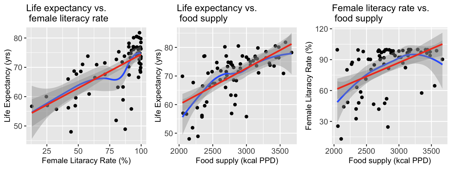
Visualize relationship in 3-D
Poll Everywhere Question 1
Learning Objectives
- Understand the population multiple linear regression model through equations and visuals.
- Fit MLR model (in
R) and understand the difference between fitted regression plane and regression lines.
- Interpret MLR (population) coefficient estimates with additional variable in model
- Based off of previous SLR work, understand how the population MLR is estimated.
How do we fit a multiple linear regression model in R?
New population model for example:
\[\text{LE} = \beta_0 + \beta_1 \text{FLR} + \beta_2 \text{FS} + \epsilon\]
# Fit regression model:
mr1 <- gapm_sub %>%
  lm(formula = LifeExpectancyYrs ~ FemaleLiteracyRate + FoodSupplykcPPD)
tidy(mr1, conf.int=T) %>% gt() %>% tab_options(table.font.size = 35) %>% fmt_number(decimals = 3)| term | estimate | std.error | statistic | p.value | conf.low | conf.high |
|---|---|---|---|---|---|---|
| (Intercept) | 33.595 | 4.472 | 7.512 | 0.000 | 24.674 | 42.517 |
| FemaleLiteracyRate | 0.157 | 0.032 | 4.873 | 0.000 | 0.093 | 0.221 |
| FoodSupplykcPPD | 0.008 | 0.002 | 4.726 | 0.000 | 0.005 | 0.012 |
Fitted multiple regression model:
\[\begin{aligned} \widehat{\text{LE}} &= \widehat{\beta}_0 + \widehat{\beta}_1 \text{FLR} + \widehat{\beta}_2 \text{FS} \\ \widehat{\text{LE}} &= 33.595 + 0.157 \ \text{FLR} + 0.008\ \text{FS} \end{aligned}\]
Don’t forget summary() to extract information!
Call:
lm(formula = LifeExpectancyYrs ~ FemaleLiteracyRate + FoodSupplykcPPD,
    data = .)

Residuals:
    Min      1Q  Median      3Q     Max
-17.715  -2.328   1.052   3.022   9.083

Coefficients:
                    Estimate Std. Error t value Pr(>|t|)
(Intercept)        33.595479   4.472049   7.512 1.56e-10 ***
FemaleLiteracyRate  0.156699   0.032158   4.873 6.75e-06 ***
FoodSupplykcPPD     0.008482   0.001795   4.726 1.17e-05 ***
---
Signif. codes:  0 '***' 0.001 '**' 0.01 '*' 0.05 '.' 0.1 ' ' 1

Residual standard error: 5.391 on 69 degrees of freedom
Multiple R-squared:  0.563, Adjusted R-squared:  0.5503
F-statistic: 44.44 on 2 and 69 DF,  p-value: 3.958e-13
Visualize the fitted multiple regression model
- The fitted model equation \[\widehat{Y} = \widehat{\beta}_0 + \widehat{\beta}_1 \cdot X_1 + \widehat{\beta}_2 \cdot X_2\] has three variables (\(Y, X_1,\) and \(X_2\)) and thus we need 3 dimensions to plot it
- Instead of a regression line, we get a regression plane
- See code in
.qmd- file. I hid it from view in the html file.
- See code in
Regression lines for varying values of food supply
\[\begin{aligned} \widehat{\text{LE}} &= \widehat{\beta}_0 + \widehat{\beta}_1 \text{FLR} + \widehat{\beta}_2 \text{FS} \\ \widehat{\text{LE}} &= 33.595 + 0.157 \ \text{FLR} + 0.008\ \text{FS} \end{aligned}\]
How do we calculate the regression line for 3000 kc PPD food supply?
\[\begin{aligned} \widehat{\text{LE}} &= 33.595 + 0.157 \ \text{FLR} + 0.008\ \text{FS}\\ \widehat{\text{LE}} &= 33.595 + 0.157 \ \text{FLR} + 0.008\cdot 3000\\ \widehat{\text{LE}} &= 33.595 + 0.157 \ \text{FLR} + 25.446 \\ \widehat{\text{LE}} &= 59.042 + 0.157 \ \text{FLR} \end{aligned}\]
Poll Everwhere Question 2
Learning Objectives
- Understand the population multiple linear regression model through equations and visuals.
- Fit MLR model (in
R) and understand the difference between fitted regression plane and regression lines.
- Interpret MLR (population) coefficient estimates with additional variable in model
- Based off of previous SLR work, understand how the population MLR is estimated.
Interpreting the estimated population coefficients
- For a population model: \[Y = \beta_0 + \beta_1 X_1 + \beta_2 X_2+ \epsilon\]
- Where \(X_1\) and \(X_2\) are continuous variables
- No need to specify \(Y\) because it required to be continuous in linear regression
General interpretation for \(\widehat{\beta}_0\)
The expected \(Y\)-variable is (\(\widehat\beta_0\) units) when the \(X_1\)-variable is 0 \(X_1\)-units and \(X_2\)-variable is 0 \(X_1\)-units (95% CI: LB, UB).
General interpretation for \(\widehat{\beta}_1\)
For every increase of 1 \(X_1\)-unit in the \(X_1\)-variable, adjusting/controlling for \(X_2\)-variable, there is an expected increase/decrease of \(|\widehat\beta_1|\) units in the \(Y\)-variable (95%: LB, UB).
General interpretation for \(\widehat{\beta}_2\)
For every increase of 1 \(X_2\)-unit in the \(X_2\)-variable, adjusting/controlling for \(X_1\)-variable, there is an expected increase/decrease of \(|\widehat\beta_2|\) units in the \(Y\)-variable (95%: LB, UB).
Interpreting the estimated population coefficient: \(\widehat{\beta}_0\)
- For an estimated model: \(\widehat{Y} = \widehat{\beta}_0 + \widehat{\beta}_1 X_2 + \widehat{\beta}_2 X_2\)
\[\begin{aligned} \widehat{Y} = &\widehat{\beta}_0 + \widehat{\beta}_1 0 + \widehat{\beta}_2 0\\ \widehat{Y} = &\widehat{\beta}_0 \\ \end{aligned}\]
Interpretation: The expected \(Y\)-variable is (\(\widehat\beta_0\) units) when the \(X_1\)-variable is 0 \(X_1\)-units and \(X_2\)-variable is 0 \(X_1\)-units (95% CI: LB, UB).
Interpreting the estimated population coefficient: \(\widehat{\beta}_1\)
We will use: \(x_{1a}\) and \(x_{1b} = x_{1a} + 1\), with the implication that \(\Delta{x_1} = x_{1b} - x_{1a} = 1\)
Our goal is to get to a statement with \(\widehat{\beta}_1\) alone:
\[\begin{aligned} \widehat{Y}|x_{1a} = &\widehat{\beta}_0 + \widehat{\beta}_1 x_{1a} + \widehat{\beta}_2 X_2\\ \widehat{Y}|x_{1b} = &\widehat{\beta}_0 + \widehat{\beta}_1 x_{1b} + \widehat{\beta}_2 X_2\\ \widehat{Y}|x_{1b} - \widehat{Y}|x_{1a} = & \bigg[\widehat{\beta}_0 + \widehat{\beta}_1 x_{1b} + \widehat{\beta}_2 X_2\bigg] - \bigg[\widehat{\beta}_0 + \widehat{\beta}_1 x_{1a} + \widehat{\beta}_2 X_2\bigg] \\ \widehat{Y}|x_{1b} - \widehat{Y}|x_{1a} = & \widehat{\beta}_1 x_{1b} - \widehat{\beta}_1 x_{1a}\\ \widehat{Y}|x_{1b} - \widehat{Y}|x_{1a} = & \widehat{\beta}_1 (x_{1b} - x_{1a})\\ \widehat{Y}|x_{1b} - \widehat{Y}|x_{1a} = & \widehat{\beta}_1\\ \end{aligned}\]
Interpretation: For every increase of 1 \(X_1\)-unit in the \(X_1\)-variable, adjusting/controlling for \(X_2\)-variable, there is an expected increase/decrease of \(|\widehat\beta_1|\) units in the \(Y\)-variable (95%: LB, UB).
Interpreting the estimated population coefficient: \(\widehat{\beta}_2\)
We can so the same for \(X_2\): \(x_{2a}\) and \(x_{2b} = x_{2a} + 1\), with the implication that \(\Delta{x_2} = x_{2b} - x_{2a} = 1\)
Our goal is to get to a statement with \(\widehat{\beta}_1\) alone:
\[\begin{aligned} \widehat{Y}|x_{2a} = &\widehat{\beta}_0 + \widehat{\beta}_1 x_{1a} + \widehat{\beta}_2 X_2\\ \widehat{Y}|x_{2b} = &\widehat{\beta}_0 + \widehat{\beta}_1 x_{1b} + \widehat{\beta}_2 X_2\\ \widehat{Y}|x_{2b} - \widehat{Y}|x_{2a} = & \bigg[\widehat{\beta}_0 + \widehat{\beta}_1 X_1 + \widehat{\beta}_2 x_{2b} \bigg] - \bigg[\widehat{\beta}_0 + \widehat{\beta}_1 X_1 + \widehat{\beta}_2 x_{2a}\bigg] \\ \widehat{Y}|x_{2b} - \widehat{Y}|x_{2a} = & \widehat{\beta}_2 x_{2b} - \widehat{\beta}_2 x_{2a}\\ \widehat{Y}|x_{2b} - \widehat{Y}|x_{2a} = & \widehat{\beta}_2 (x_{2b} - x_{2a})\\ \widehat{Y}|x_{2b} - \widehat{Y}|x_{2a} = & \widehat{\beta}_2\\ \end{aligned}\]
Interpretation: For every increase of 1 \(X_2\)-unit in the \(X_2\)-variable, adjusting/controlling for \(X_1\)-variable, there is an expected increase/decrease of \(|\widehat\beta_2|\) units in the \(Y\)-variable (95%: LB, UB).
Poll Everywhere Question 3
Getting these interpretations from our regression table
We fit the regression model in R and printed the regression table:
| term | estimate | std.error | statistic | p.value | conf.low | conf.high |
|---|---|---|---|---|---|---|
| (Intercept) | 33.595 | 4.472 | 7.512 | 0.000 | 24.674 | 42.517 |
| FemaleLiteracyRate | 0.157 | 0.032 | 4.873 | 0.000 | 0.093 | 0.221 |
| FoodSupplykcPPD | 0.008 | 0.002 | 4.726 | 0.000 | 0.005 | 0.012 |
Fitted multiple regression model: \(\widehat{\text{LE}} = 33.595 + 0.157 \text{ FLR} + 0.008 \text{ FS}\)
Interpretation for \(\widehat{\beta}_0\)
The average life expectancy is 33.595 years when the female literacy rate is 0% and food supply is 0 kcal PPD (95% CI: 24.674, 41.517).
Interpretation for \(\widehat{\beta}_1\)
For every 1% increase in the female literacy rate, adjusting for food supply, there is an expected increase of 0.157 years in the life expectancy (95%: 0.093, 0.221).
Interpretation for \(\widehat{\beta}_2\)
For every 1 kcal PPD increase in the food supply, adjusting for female literacy rate, there is an expected increase of 0.008 years in life expectancy (95%: 0.005, 0.012).
What we need in our interpretations of coefficients (reference)
Units of Y
Units of X
If discussing intercept: Mean or average or expected before Y
If discussing coefficient for continuous covariate: Mean or average or expected before difference, increase, or decrease
- OR: Mean or average or expected before Y
- NOT: predicted
- Only need before difference or Y!!
Confidence interval
If other covariates in the model
Discussing intercept: Must state that variables are equal to 0
- or at their centered value if centered!
Discussing coefficient for covariate: Must state “adjusting for all other variables”, “Controlling for all other variables”, or “Holding all other variables constant”
- If only one other variable in the model, then replace “all other variables” with the single variable name
Learning Objectives
- Understand the population multiple linear regression model through equations and visuals.
- Fit MLR model (in
R) and understand the difference between fitted regression plane and regression lines. - Interpret MLR (population) coefficient estimates with additional variable in model
- Based off of previous SLR work, understand how the population MLR is estimated.
How do we estimate the model parameters?
- We need to estimate the population model coefficients \(\widehat{\beta}_0, \widehat{\beta}_1, \widehat{\beta}_2, \ldots, \widehat{\beta}_k\)
- This can be done using the ordinary least-squares method
- Find the \(\widehat{\beta}\) values that minimize the sum of squares due to error (\(SSE\))
\[ \begin{aligned} SSE & = \displaystyle\sum^n_{i=1} \widehat\epsilon_i^2 \\ SSE & = \displaystyle\sum^n_{i=1} (Y_i - \widehat{Y}_i)^2 \\ SSE & = \displaystyle\sum^n_{i=1} (Y_i - (\widehat{\beta}_0 +\widehat{\beta}_1 X_{i1}+ \ldots+\widehat{\beta}_1 X_{ik}))^2 \\ SSE & = \displaystyle\sum^n_{i=1} (Y_i - \widehat{\beta}_0 -\widehat{\beta}_1 X_{i1}- \ldots-\widehat{\beta}_1 X_{ik})^2 \end{aligned}\]
Technical side note (not needed in our class)
The equations for calculating the \(\boldsymbol{\widehat{\beta}}\) values is best done using matrix notation (not required for our class)
We will be using
Rto get the coefficients instead of the equation (already did this a few slides back!)How we have represented the population regression model: \[Y = \beta_0 + \beta_1 X_1 + \beta_2 X_2+ \ldots + \beta_k X_k + \epsilon\]
- How to represent population model with matrix notation:
\[\begin{aligned} \boldsymbol{Y} &= \boldsymbol{X}\boldsymbol{\beta} + \boldsymbol{\epsilon} \\ \boldsymbol{Y}_{n \times 1}& = \boldsymbol{X}_{n \times (k+1)}\boldsymbol{\beta}_{(k+1)\times 1} + \boldsymbol{\epsilon}_{n \times 1} \end{aligned}\]
- \(\boldsymbol{X}\) is often called the design matrix
- Each row represents an individual
- Each column represents a covariate
\[ \boldsymbol{Y} = \left[\begin{array}{c} Y_1 \\ Y_2 \\ \vdots \\ Y_n \end{array} \right]_{n \times 1} \] \[ \boldsymbol{\epsilon} = \left[\begin{array}{c} \epsilon_1 \\ \epsilon_2 \\ \vdots \\ \epsilon_n \end{array} \right]_{n \times 1} \]
\[ \boldsymbol{X} = \left[ \begin{array}{ccccc} 1 & X_{11} & X_{12} & \ldots & X_{1,k} \\ 1 &X_{21} & X_{22} & \ldots & X_{2,k} \\ \vdots&\vdots & \vdots & \ldots & \vdots \\ 1 & X_{n1} & X_{n2} & \ldots & X_{n,k} \end{array} \right]_{n \times (k+1)} \]
\[ \boldsymbol{\beta} = \left[\begin{array}{c} \beta_0 \\ \beta_1\\ \vdots \\ \beta_{k} \end{array} \right]_{(k+1)\times 1} \]
LINE model assumptions
[L] Linearity of relationship between variables
The mean value of \(Y\) given any combination of \(X_1, X_2, \ldots, X_k\) values, is a linear function of \(\beta_0, \beta_1, \beta_2, \ldots, \beta_k\):
\[\mu_{Y|X_1, \ldots, X_k} = \beta_0 + \beta_1 X_1 + \beta_2 X_2+ \ldots + \beta_k X_k\]
[I] Independence of the \(Y\) values
Observations (\(X_1, X_2, \ldots, X_k, Y\)) are independent from one another
[N] Normality of the \(Y\)’s given \(X\) (residuals)
\(Y\) has a normal distribution for any any combination of \(X_1, X_2, \ldots, X_k\) values
- Thus, the residuals are normally distributed
[E] Equality of variance of the residuals (homoscedasticity)
The variance of \(Y\) is the same for any any combination of \(X_1, X_2, \ldots, X_k\) values
\[\sigma^2_{Y|X_1, X_2, \ldots, X_k} = Var(Y|X_1, X_2, \ldots, X_k) = \sigma^2\]
Summary of the LINE assumptions
- Equivalently, the residuals are independently and identically distributed (iid):
- normal
- with mean 0 and
- constant variance \(\sigma^2\)
- Residuals are still \(\widehat{\epsilon}_i=Y_i - \widehat{Y}_i\) for each observation
- It’s just that \(\widehat{Y}_i\) is now calculated with many covariates (\(X_1, X_2, \ldots, X_k\))
Variation: Explained vs. Unexplained
\[\begin{aligned} \sum_{i=1}^n (Y_i - \overline{Y})^2 &= \sum_{i=1}^n (\widehat{Y}_i- \overline{Y})^2 + \sum_{i=1}^n (Y_i - \widehat{Y}_i)^2 \\ SSY &= SSR + SSE \end{aligned}\]
- \(Y_i - \overline{Y}\) = the deviation of \(Y_i\) around the mean \(\overline{Y}\)
- the total amount deviation
- \(\widehat{Y}_i- \overline{Y}\) = the deviation of the fitted value \(\widehat{Y}_i\) around the mean \(\overline{Y}\)
- the amount deviation explained by the regression at \(X_{i1},\ldots,X_{ik}\)
- \(Y_i - \widehat{Y}_i\) = the deviation of the observation \(Y\) around the fitted regression line
- the amount deviation unexplained by the regression at \(X_{i1},\ldots,X_{ik}\)
Poll Everywhere Question 4
SLR: Another way to think of SSY, SSR, and SSE
Let’s create a data frame of each component within the SS’s
- Deviation in SSY: \(Y_i - \overline{Y}\)
- Deviation in SSR: \(\widehat{Y}_i- \overline{Y}\)
- Deviation in SSE: \(Y_i - \widehat{Y}_i\)
Using our simple linear regression model as an example:
slr1 <- gapm_sub %>%
  lm(formula = LifeExpectancyYrs ~ FemaleLiteracyRate)
aug_slr1 = augment(slr1)
SS_dev_slr = gapm_sub %>% select(LifeExpectancyYrs) %>%
  mutate(SSY_dev = LifeExpectancyYrs - mean(LifeExpectancyYrs),
         y_hat = aug_slr1$.fitted,
         SSR_dev = y_hat - mean(LifeExpectancyYrs),
SSE_dev = aug_slr1$.resid)SLR: Plot the components of each sum of squares
Code to make the below plots
SSY_plot = ggplot(SS_dev_slr, aes(SSY_dev)) + geom_histogram() + xlim(-30, 30) + ylim(0, 35) + xlab(expression(Y[i] - bar(Y)))
SSR_plot = ggplot(SS_dev_slr, aes(SSR_dev)) + geom_histogram() + xlim(-30, 30) + ylim(0, 35) +xlab(expression(hat(Y)[i] - bar(Y)))
SSE_plot = ggplot(SS_dev_slr, aes(SSE_dev)) + geom_histogram() + xlim(-30, 30) + ylim(0, 35) + xlab(expression(Y[i] - hat(Y)[i]))
grid.arrange(SSY_plot, SSR_plot, SSE_plot, nrow = 3)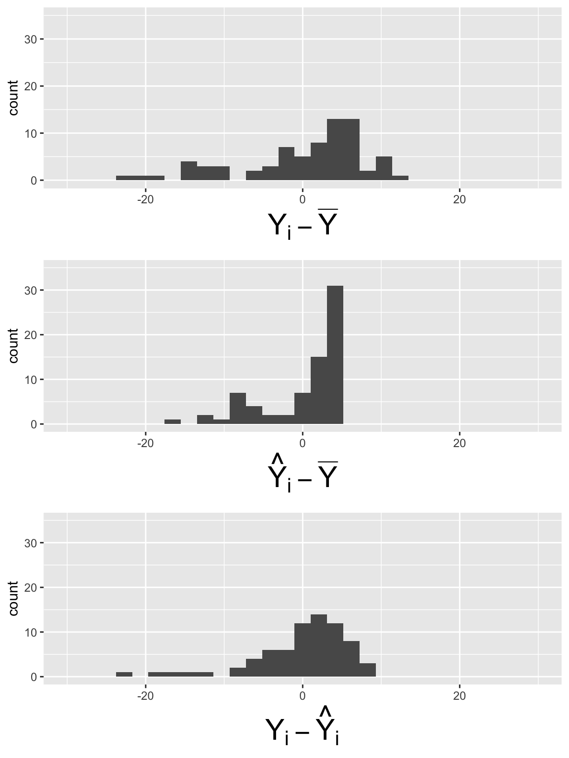
\[SSY = \sum_{i=1}^n (Y_i - \overline{Y})^2 = 64.64\]
\[SSR = \sum_{i=1}^n (\widehat{Y}_i- \overline{Y})^2 = 27.24\]
\[SSE =\sum_{i=1}^n (Y_i - \widehat{Y}_i)^2 = 37.39\]
MLR: Another way to think of SSY, SSR, and SSE
Let’s create a data frame of each component within the SS’s
- Deviation in SSY: \(Y_i - \overline{Y}\)
- Deviation in SSR: \(\widehat{Y}_i- \overline{Y}\)
- Deviation in SSE: \(Y_i - \widehat{Y}_i\)
Using our simple linear regression model as an example:
mr1 <- gapm_sub %>%
  lm(formula = LifeExpectancyYrs ~ FemaleLiteracyRate + FoodSupplykcPPD)
aug_mlr1 = augment(mr1)
SS_df = gapm_sub %>% select(LifeExpectancyYrs) %>%
  mutate(SSY_dev = LifeExpectancyYrs - mean(LifeExpectancyYrs),
         y_hat = aug_mlr1$.fitted,
         SSR_dev = y_hat - mean(LifeExpectancyYrs),
         SSE_dev = aug_mlr1$.resid)
MLR: Plot the components of each sum of squares
Code to make the below plots
SSY_plot = ggplot(SS_df, aes(SSY_dev)) + geom_histogram() + xlim(-30, 30) + ylim(0, 35) + xlab(expression(Y[i] - bar(Y)))
SSR_plot = ggplot(SS_df, aes(SSR_dev)) + geom_histogram() + xlim(-30, 30) + ylim(0, 35) +xlab(expression(hat(Y)[i] - bar(Y)))
SSE_plot = ggplot(SS_df, aes(SSE_dev)) + geom_histogram() + xlim(-30, 30) + ylim(0, 35) + xlab(expression(Y[i] - hat(Y)[i]))
grid.arrange(SSY_plot, SSR_plot, SSE_plot, nrow = 3)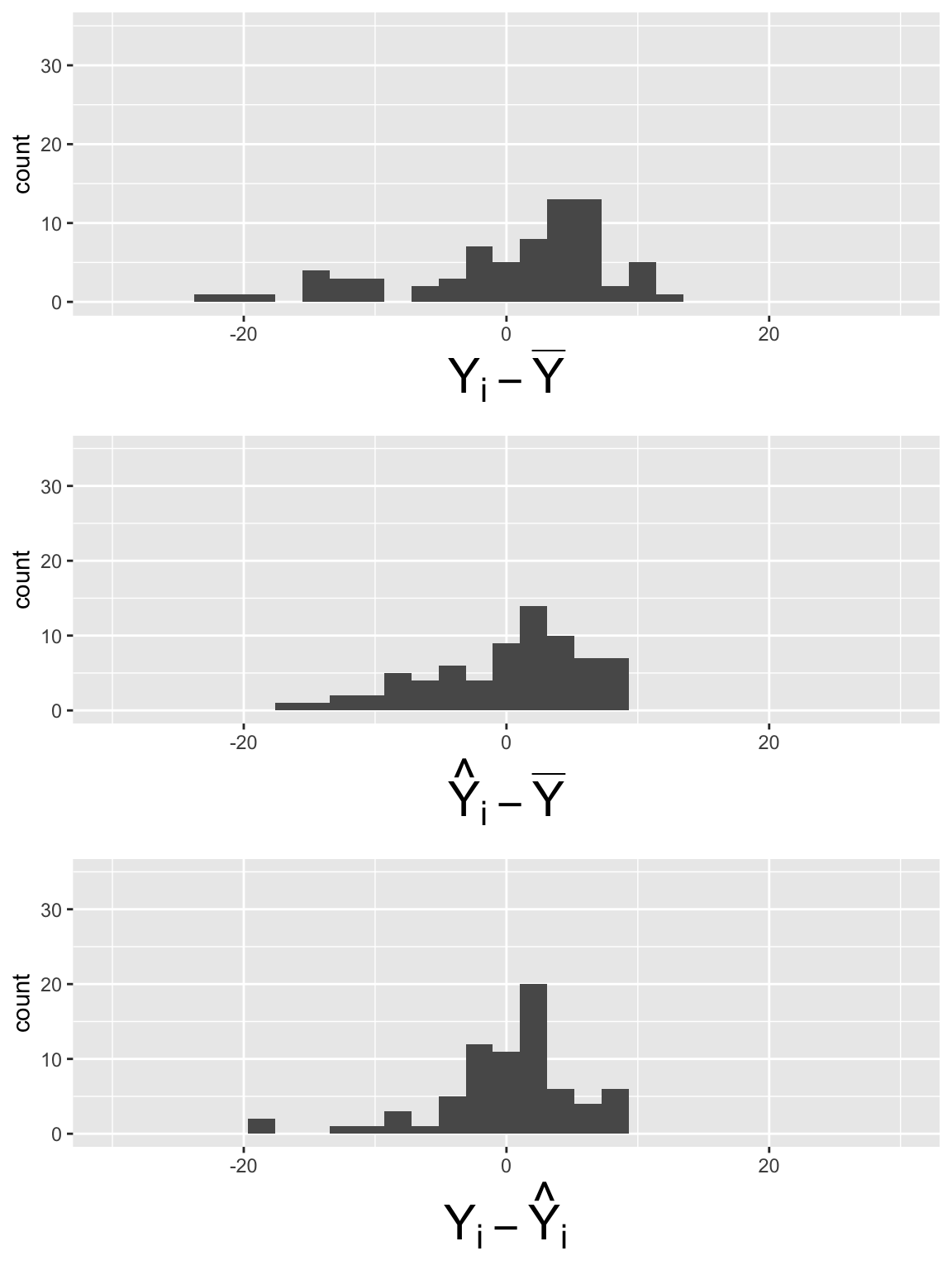
\[SSY = \sum_{i=1}^n (Y_i - \overline{Y})^2 = 64.64\]
\[SSR = \sum_{i=1}^n (\widehat{Y}_i- \overline{Y})^2 = 36.39\]
\[SSE =\sum_{i=1}^n (Y_i - \widehat{Y}_i)^2 = 28.25\]
What did you notice in the plots?
Simple Linear Regression
Multiple Linear Regression

\[SSY = 64.64\]
\[SSR = 27.24\]
\[SSE =37.39\]

\[SSY = 64.64\]
\[SSR = 36.39\]
\[SSE =28.25\]
- Next class: we can determine if model fit is better by comparing the SSE’s of different models
Lesson 9: MLR Intro