Lesson 12: Interactions, Part 2
Nicky Wakim
2025-02-19
Learning Objectives
Last time:
- Define confounders and effect modifiers, and how they interact with the main relationship we model.
- Interpret the interaction component of a model with a binary categorical covariate and continuous covariate, and how the main variable’s effect changes.
- Interpret the interaction component of a model with a multi-level categorical covariate and continuous covariate, and how the main variable’s effect changes.
This time:
- Interpret the interaction component of a model with two categorical covariates, and how the main variable’s effect changes.
- Interpret the interaction component of a model with two continuous covariates, and how the main variable’s effect changes.
- Report results for a best-fit line (with confidence intervals) at different levels of an effect measure modifier
Learning Objectives
Last time:
- Define confounders and effect modifiers, and how they interact with the main relationship we model.
- Interpret the interaction component of a model with a binary categorical covariate and continuous covariate, and how the main variable’s effect changes.
- Interpret the interaction component of a model with a multi-level categorical covariate and continuous covariate, and how the main variable’s effect changes.
This time:
- Interpret the interaction component of a model with two categorical covariates, and how the main variable’s effect changes.
- Interpret the interaction component of a model with two continuous covariates, and how the main variable’s effect changes.
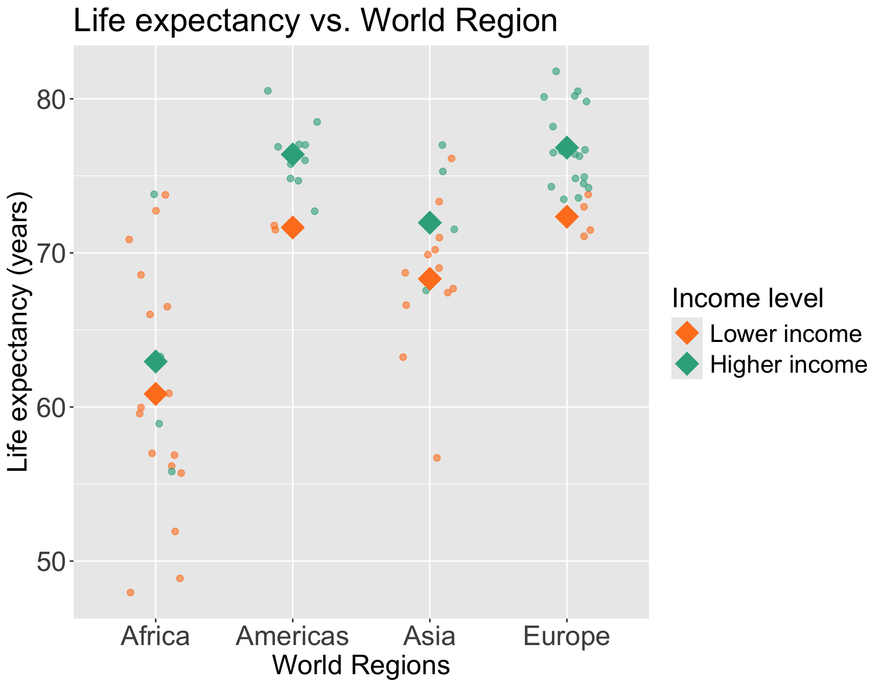
Do we think income level can be an effect modifier for world region?
Taking a break from female literacy rate to demonstrate interactions for two categorical variables
We can start by visualizing the relationship between life expectancy and world region by income level
Questions of interest: Does the effect of world region on life expectancy differ depending on income level?
- This is the same as: Is income level an effect modifier for world region?
Let’s run an interaction model to see!
Model with interaction between a multi-level categorical and binary variables
Model we are fitting:
\[\begin{aligned}LE = &\beta_0 + \beta_1 I(\text{high income}) + \beta_2 I(\text{Americas}) + \beta_3 I(\text{Asia}) + \beta_4 I(\text{Europe}) + \\ & \beta_5 \cdot I(\text{high income}) \cdot I(\text{Americas}) + \beta_6\cdot I(\text{high income}) \cdot I(\text{Asia})+ \\ & \beta_7 \cdot I(\text{high income})\cdot I(\text{Europe})+ \epsilon \end{aligned}\]
- \(LE\) as life expectancy
- \(I(\text{high income})\) as indicator of high income
- \(I(\text{Americas})\), \(I(\text{Asia})\), \(I(\text{Europe})\) as the indicator for each world region
In R:
# gapm_sub = gapm_sub %>% mutate(income_levels2 = relevel(income_levels2, ref = "Higher income")) # for poll everywhere

m_int_wr_inc = lm(LifeExpectancyYrs ~ income_levels2 + four_regions +
                  income_levels2*four_regions, data = gapm_sub)
m_int_wr_inc = lm(LifeExpectancyYrs ~ income_levels2*four_regions,
                data = gapm_sub)
Displaying the regression table and writing fitted regression equation
tidy(m_int_wr_inc, conf.int=T) %>% gt() %>% tab_options(table.font.size = 25) %>% fmt_number(decimals = 3)| term | estimate | std.error | statistic | p.value | conf.low | conf.high |
|---|---|---|---|---|---|---|
| (Intercept) | 60.850 | 1.281 | 47.488 | 0.000 | 58.290 | 63.410 |
| income_levels2Higher income | 2.100 | 2.865 | 0.733 | 0.466 | −3.624 | 7.824 |
| four_regionsAmericas | 10.800 | 3.844 | 2.810 | 0.007 | 3.121 | 18.479 |
| four_regionsAsia | 7.467 | 1.957 | 3.815 | 0.000 | 3.556 | 11.377 |
| four_regionsEurope | 11.500 | 2.865 | 4.014 | 0.000 | 5.776 | 17.224 |
| income_levels2Higher income:four_regionsAmericas | 2.640 | 4.896 | 0.539 | 0.592 | −7.141 | 12.421 |
| income_levels2Higher income:four_regionsAsia | 1.543 | 3.956 | 0.390 | 0.698 | −6.360 | 9.447 |
| income_levels2Higher income:four_regionsEurope | 2.382 | 4.020 | 0.592 | 0.556 | −5.649 | 10.412 |
\[\begin{aligned} \widehat{LE} = &\widehat\beta_0 + \widehat\beta_1 I(\text{high income}) + \widehat\beta_2 I(\text{Americas}) + \widehat\beta_3 I(\text{Asia}) + \widehat\beta_4 I(\text{Europe}) + \\ & \widehat\beta_5 \cdot I(\text{high income}) \cdot I(\text{Americas}) + \widehat\beta_6\cdot I(\text{high income}) \cdot I(\text{Asia})+ \\ & \widehat\beta_7 \cdot I(\text{high income})\cdot I(\text{Europe}) \\ \widehat{LE} = & 60.85 + 2.10 \cdot I(\text{high income}) + 10.8 \cdot I(\text{Americas}) + 7.47\cdot I(\text{Asia}) + 11.50 \cdot I(\text{Europe}) + \\ & 2.64 \cdot I(\text{high income}) \cdot I(\text{Americas}) + 1.54 \cdot I(\text{high income}) \cdot I(\text{Asia})+ \\ & 2.38 \cdot I(\text{high income})\cdot I(\text{Europe}) \\ \end{aligned}\]
Poll Everywhere Question 4
Comparing fitted regression means for each world region
\[\begin{aligned} \widehat{LE} = &\widehat\beta_0 + \widehat\beta_1 I(\text{high income}) + \widehat\beta_2 I(\text{Americas}) + \widehat\beta_3 I(\text{Asia}) + \widehat\beta_4 I(\text{Europe}) + \\ & \widehat\beta_5 \cdot I(\text{high income}) \cdot I(\text{Americas}) + \widehat\beta_6\cdot I(\text{high income}) \cdot I(\text{Asia})+ \\ & \widehat\beta_7 \cdot I(\text{high income})\cdot I(\text{Europe}) \\ \widehat{LE} = & 60.85 + 2.10 \cdot I(\text{high income}) + 10.8 \cdot I(\text{Americas}) + 7.47\cdot I(\text{Asia}) + 11.50 \cdot I(\text{Europe}) + \\ & 2.64 \cdot I(\text{high income}) \cdot I(\text{Americas}) + 1.54 \cdot I(\text{high income}) \cdot I(\text{Asia})+ \\ & 2.38 \cdot I(\text{high income})\cdot I(\text{Europe}) \\ \end{aligned}\]
Africa
\[\begin{aligned} \widehat{LE} = &\widehat\beta_0 + \widehat\beta_1 I(\text{high income}) + \\ & \widehat\beta_2 \cdot 0 + \widehat\beta_3 \cdot 0 + \widehat\beta_4 \cdot 0 + \\ & \widehat\beta_5 I(\text{high income}) \cdot 0 + \\ & \widehat\beta_6 I(\text{high income}) \cdot 0+ \\& \widehat\beta_7 I(\text{high income}) \cdot 0 \\ \widehat{LE} = &\widehat\beta_0 + \widehat\beta_1 I(\text{high income})\\ \end{aligned}\]
The Americas
\[\begin{aligned} \widehat{LE} = &\widehat\beta_0 + \widehat\beta_1 I(\text{high income}) + \\ & \widehat\beta_2 \cdot 1 + \widehat\beta_3 \cdot 0 + \widehat\beta_4 \cdot 0 + \\ & \widehat\beta_5 I(\text{high income}) \cdot 1 + \\ & \widehat\beta_6 I(\text{high income}) \cdot 0+ \\ & \widehat\beta_7 I(\text{high income}) \cdot 0 \\ \widehat{LE} = &\big(\widehat\beta_0+\widehat\beta_2\big) + \\ &\big(\widehat\beta_1 + \widehat\beta_5\big)I(\text{high income}) \\ \end{aligned}\]
Asia
\[\begin{aligned} \widehat{LE} = &\widehat\beta_0 + \widehat\beta_1 I(\text{high income}) + \\ & \widehat\beta_2 \cdot 0 + \widehat\beta_3 \cdot 1 + \widehat\beta_4 \cdot 0 + \\ & \widehat\beta_5 I(\text{high income}) \cdot 0 + \\ & \widehat\beta_6 I(\text{high income}) \cdot 1+ \\ & \widehat\beta_7 I(\text{high income}) \cdot 0 \\ \widehat{LE} = &\big(\widehat\beta_0+\widehat\beta_3\big) + \\ &\big(\widehat\beta_1 + \widehat\beta_6\big)I(\text{high income}) \\ \end{aligned}\]
Europe
\[\begin{aligned} \widehat{LE} = &\widehat\beta_0 + \widehat\beta_1 I(\text{high income}) + \\ & \widehat\beta_2 \cdot 0 + \widehat\beta_3 \cdot 0 + \widehat\beta_4 \cdot 1 + \\ & \widehat\beta_5 I(\text{high income}) \cdot 0 + \\ & \widehat\beta_6 I(\text{high income}) \cdot 0+ \\ & \widehat\beta_7 I(\text{high income}) \cdot 1 \\ \widehat{LE} = &\big(\widehat\beta_0+\widehat\beta_4\big) + \\ & \big(\widehat\beta_1 + \widehat\beta_7\big)I(\text{high income}) \\ \end{aligned}\]
Comparing fitted regression means for each income level
\[\begin{aligned} \widehat{LE} = &\widehat\beta_0 + \widehat\beta_1 I(\text{high income}) + \widehat\beta_2 I(\text{Americas}) + \widehat\beta_3 I(\text{Asia}) + \widehat\beta_4 I(\text{Europe}) + \\ & \widehat\beta_5 \cdot I(\text{high income}) \cdot I(\text{Americas}) + \widehat\beta_6\cdot I(\text{high income}) \cdot I(\text{Asia})+ \\ & \widehat\beta_7 \cdot I(\text{high income})\cdot I(\text{Europe}) \\ \widehat{LE} = & 60.85 + 2.10 \cdot I(\text{high income}) + 10.8 \cdot I(\text{Americas}) + 7.47\cdot I(\text{Asia}) + 11.50 \cdot I(\text{Europe}) + \\ & 2.64 \cdot I(\text{high income}) \cdot I(\text{Americas}) + 1.54 \cdot I(\text{high income}) \cdot I(\text{Asia})+ \\ & 2.38 \cdot I(\text{high income})\cdot I(\text{Europe}) \\ \end{aligned}\]
For lower income countries: \(I(\text{high income}) =0\)
\[ \begin{aligned} \widehat{LE} = &\widehat\beta_0 + \widehat\beta_1 \cdot 0 + \widehat\beta_2 I(\text{Americas}) + \widehat\beta_3 I(\text{Asia}) + \widehat\beta_4 I(\text{Europe}) + \\ & \widehat\beta_5 \cdot 0\cdot I(\text{Americas}) + \widehat\beta_6\cdot 0 \cdot I(\text{Asia})+ \widehat\beta_7 \cdot 0\cdot I(\text{Europe}) \\ \widehat{LE} = &\widehat\beta_0 + \widehat\beta_2 I(\text{Americas}) + \widehat\beta_3 I(\text{Asia}) + \widehat\beta_4 I(\text{Europe}) \\ \end{aligned}\]
For higher income countries: \(I(\text{high income}) =1\)
\[ \begin{aligned} \widehat{LE} = &\widehat\beta_0 + \widehat\beta_1 \cdot 1 + \widehat\beta_2 I(\text{Americas}) + \widehat\beta_3 I(\text{Asia}) + \widehat\beta_4 I(\text{Europe}) + \\ & \widehat\beta_5 \cdot 1\cdot I(\text{Americas}) + \widehat\beta_6\cdot 1 \cdot I(\text{Asia})+ \widehat\beta_7 \cdot 1\cdot I(\text{Europe}) \\ \widehat{LE} = & (\widehat\beta_0 + \widehat\beta_1) + (\widehat\beta_2 + \widehat\beta_5) I(\text{Americas}) + (\widehat\beta_3 + \widehat\beta_6) I(\text{Asia}) + \\ & (\widehat\beta_4 + \widehat\beta_7) I(\text{Europe}) \\ \end{aligned}\]
- Example interpretation: The America’s effect on mean life expectancy increases \(\widehat{\beta}_5\) comparing high income to low income countries.
Let’s take a look back at the plot
For lower income countries: \(I(\text{high income}) =0\)
\[ \begin{aligned} \widehat{LE} = &\widehat\beta_0 + \widehat\beta_2 I(\text{Americas}) + \widehat\beta_3 I(\text{Asia}) + \\ & \widehat\beta_4 I(\text{Europe}) \\ \end{aligned}\]
For higher income countries: \(I(\text{high income}) =1\)
\[ \begin{aligned} \widehat{LE} = & (\widehat\beta_0 + \widehat\beta_1) + (\widehat\beta_2 + \widehat\beta_5) I(\text{Americas}) + \\& (\widehat\beta_3 + \widehat\beta_6) I(\text{Asia}) + (\widehat\beta_4 + \widehat\beta_7) I(\text{Europe}) \\ \end{aligned}\]
Interpretation for interaction between two categorical variables
\[ \begin{aligned} \widehat{LE} = &\widehat\beta_0 + \widehat\beta_1 \cdot I(\text{high income}) + \widehat\beta_2 I(\text{Americas}) + \widehat\beta_3 I(\text{Asia}) + \widehat\beta_4 I(\text{Europe}) + \\ & \widehat\beta_5 \cdot I(\text{high income})\cdot I(\text{Americas}) + \widehat\beta_6\cdot I(\text{high income}) \cdot I(\text{Asia})+ \\ & \widehat\beta_7 \cdot I(\text{high income})\cdot I(\text{Europe}) \\ \widehat{LE} = & \bigg[\widehat\beta_0 + \widehat\beta_1 \cdot I(\text{high income})\bigg] + \bigg[\widehat\beta_2 + \widehat\beta_5 \cdot I(\text{high income})\bigg] I(\text{Americas}) + \\ & \bigg[\widehat\beta_3 + \widehat\beta_6 \cdot I(\text{high income})\bigg] I(\text{Asia}) + \bigg[\widehat\beta_4 + \widehat\beta_7 \cdot I(\text{high income})\bigg] I(\text{Europe}) \\ \end{aligned}\]
- Interpretation:
- \(\beta_1\) = mean change in the Africa’s life expectancy, comparing high income to low income countries
- \(\beta_5\) = mean change in the Americas’ effect, comparing high income to low income countries
- \(\beta_6\) = mean change in Asia’s effect, comparing high income to low income countries
- \(\beta_7\) = mean change in Europe’s effect, comparing high income to low income countries
Test interaction between two categorical variables (1/2)
- We run an F-test for a group of coefficients (\(\beta_5\), \(\beta_6\), \(\beta_7\)) in the below model (see lesson 9)
\[\begin{aligned}LE = &\beta_0 + \beta_1 I(\text{high income}) + \beta_2 I(\text{Americas}) + \beta_3 I(\text{Asia}) + \beta_4 I(\text{Europe}) + \\ & \beta_5 \cdot I(\text{high income}) \cdot I(\text{Americas}) + \beta_6\cdot I(\text{high income}) \cdot I(\text{Asia})+ \\ & \beta_7 \cdot I(\text{high income})\cdot I(\text{Europe})+ \epsilon \end{aligned}\]
Null \(H_0\)
\(\beta_5= \beta_6 = \beta_7 =0\)
Alternative \(H_1\)
\(\beta_5\neq0\) and/or \(\beta_6\neq0\) and/or \(\beta_7\neq0\)
Null / Smaller / Reduced model
\[\begin{aligned}LE = &\beta_0 + \beta_1 I(\text{high income}) + \beta_2 I(\text{Americas}) + \\& \beta_3 I(\text{Asia}) + \beta_4 I(\text{Europe}) + \epsilon \end{aligned}\]
Alternative / Larger / Full model
\[\begin{aligned}LE = &\beta_0 + \beta_1 I(\text{high income}) + \beta_2 I(\text{Americas}) + \beta_3 I(\text{Asia}) + \\ & \beta_4 I(\text{Europe}) + \beta_5 \cdot I(\text{high income}) \cdot I(\text{Americas}) + \\ & \beta_6\cdot I(\text{high income}) \cdot I(\text{Asia})+ \beta_7 \cdot I(\text{high income})\cdot I(\text{Europe})+ \epsilon \end{aligned}\]
Test interaction between two categorical variables (2/2)
- Fit the reduced and full model
- Display the ANOVA table with F-statistic and p-value
| term | df.residual | rss | df | sumsq | statistic | p.value |
|---|---|---|---|---|---|---|
| LifeExpectancyYrs ~ income_levels2 + four_regions | 67.000 | 1,693.242 | NA | NA | NA | NA |
| LifeExpectancyYrs ~ income_levels2 + four_regions + income_levels2 * four_regions | 64.000 | 1,681.304 | 3.000 | 11.938 | 0.151 | 0.928 |
- Conclusion: There is not a significant interaction between world region and income level (p = 0.928).
Learning Objectives
Last time:
- Define confounders and effect modifiers, and how they interact with the main relationship we model.
- Interpret the interaction component of a model with a binary categorical covariate and continuous covariate, and how the main variable’s effect changes.
- Interpret the interaction component of a model with a multi-level categorical covariate and continuous covariate, and how the main variable’s effect changes.
This time:
- Interpret the interaction component of a model with two categorical covariates, and how the main variable’s effect changes.
- Interpret the interaction component of a model with two continuous covariates, and how the main variable’s effect changes.
Do we think food supply is an effect modifier for female literacy rate?
We can start by visualizing the relationship between life expectancy and female literacy rate by food supply
Questions of interest: Does the effect of female literacy rate on life expectancy differ depending on food supply?
- This is the same as: Is food supply is an effect modifier for female literacy rate? Is food supply an effect modifier of the association between life expectancy and female literacy rate?
Let’s run an interaction model to see!
Model with interaction between two continuous variables
Model we are fitting:
\[ LE = \beta_0 + \beta_1 FLR^c + \beta_2 FS^c + \beta_3 FLR^c \cdot FS^c + \epsilon\]
- \(LE\) as life expectancy
- \(FLR^c\) as the centered around the mean female literacy rate (continuous variable)
- \(FS^c\) as the centered around the mean food supply (continuous variable)
In R:
OR
Displaying the regression table and writing fitted regression equation
tidy_m_fs = tidy(m_int_fs, conf.int=T)
tidy_m_fs %>% gt() %>% tab_options(table.font.size = 35) %>% fmt_number(decimals = 5)| term | estimate | std.error | statistic | p.value | conf.low | conf.high |
|---|---|---|---|---|---|---|
| (Intercept) | 70.32060 | 0.72393 | 97.13721 | 0.00000 | 68.87601 | 71.76518 |
| FLR_c | 0.15532 | 0.03808 | 4.07905 | 0.00012 | 0.07934 | 0.23130 |
| FS_c | 0.00849 | 0.00182 | 4.67908 | 0.00001 | 0.00487 | 0.01212 |
| FLR_c:FS_c | −0.00001 | 0.00008 | −0.06908 | 0.94513 | −0.00016 | 0.00015 |
\[ \begin{aligned} \widehat{LE} = & \widehat\beta_0 + \widehat\beta_1 FLR^c + \widehat\beta_2 FS^c + \widehat\beta_3 FLR^c \cdot FS^c \\ \widehat{LE} = & 70.32 + 0.16 \cdot FLR^c + 0.01 \cdot FS^c - 0.00001 \cdot FLR^c \cdot FS^c \end{aligned}\]
Comparing fitted regression lines for various food supply values
\[ \begin{aligned} \widehat{LE} = & \widehat\beta_0 + \widehat\beta_1 FLR^c + \widehat\beta_2 FS^c + \widehat\beta_3 FLR^c \cdot FS^c \\ \widehat{LE} = & 70.32 + 0.16 \cdot FLR^c + 0.01 \cdot FS^c - 0.00001 \cdot FLR^c \cdot FS^c \end{aligned}\]
To identify different lines, we need to pick example values of Food Supply:
Food Supply of 1812 kcal PPD
\[\begin{aligned} \widehat{LE} = & \widehat\beta_0 + \widehat\beta_1 FLR^c + \\ & \widehat\beta_2 \cdot (-1000) + \\ & \widehat\beta_3 FLR^c \cdot (-1000) \\ \widehat{LE} = & \big(\widehat\beta_0 - 1000 \widehat\beta_2 \big)+ \\ & \big(\widehat\beta_1 - 1000 \widehat\beta_3 \big) FLR^c \end{aligned}\]
Food Supply of 2812 kcal PPD
\[\begin{aligned} \widehat{LE} = & \widehat\beta_0 + \widehat\beta_1 FLR^c + \\ & \widehat\beta_2 \cdot 0 + \\ & \widehat\beta_3 FLR^c \cdot 0 \\ \widehat{LE} = & \big(\widehat\beta_0 \big)+ \\ & \big(\widehat\beta_1 \big) FLR^c \end{aligned}\]
Food Supply of 3812 kcal PPD
\[\begin{aligned} \widehat{LE} = & \widehat\beta_0 + \widehat\beta_1 FLR^c + \\ & \widehat\beta_2 \cdot 1000 + \\ & \widehat\beta_3 FLR^c \cdot 1000 \\ \widehat{LE} = & \big(\widehat\beta_0 + 1000 \widehat\beta_2 \big)+ \\ & \big(\widehat\beta_1 + 1000 \widehat\beta_3 \big) FLR^c \end{aligned}\]
Poll Everywhere Question??
Interpretation for interaction between two continuous variables
\[ \begin{aligned} \widehat{LE} = & \widehat\beta_0 + \widehat\beta_1 FLR^c + \widehat\beta_2 FS^c + \widehat\beta_3 FLR^c \cdot FS^c \\ \widehat{LE} = & \bigg[\widehat\beta_0 + \widehat\beta_2 \cdot FS^c \bigg] + \underbrace{\bigg[\widehat\beta_1 + \widehat\beta_3 \cdot FS^c \bigg]}_\text{FLR's effect} FLR \\ \end{aligned}\]
Interpretation:
- \(\beta_3\) = mean change in female literacy rate’s effect, for every one kcal PPD increase in food supply
In summary, the interaction term can be interpreted as “difference in adjusted female literacy rate effect for every 1 kcal PPD increase in food supply”
It will be helpful to test the interaction to round out this interpretation!!
Test interaction between two continuous variables
- We run an F-test for a single coefficients (\(\beta_3\)) in the below model (see lesson 9)
\[ LE = \beta_0 + \beta_1 FLR^c + \beta_2 FS^c + \beta_3 FLR^c \cdot FS^c + \epsilon\]
Null \(H_0\)
\[\beta_3=0\]
Alternative \(H_1\)
\[\beta_3\neq0\]
Null / Smaller / Reduced model
\[ LE = \beta_0 + \beta_1 FLR^c + \beta_2 FS^c + \epsilon\]
Alternative / Larger / Full model
\[\begin{aligned} LE = & \beta_0 + \beta_1 FLR^c + \beta_2 FS^c + \\ & \beta_3 FLR^c \cdot FS^c + \epsilon \end{aligned}\]
Test interaction between two continuous variables
- Fit the reduced and full model
Display the ANOVA table with F-statistic and p-value
| term | df.residual | rss | df | sumsq | statistic | p.value |
|---|---|---|---|---|---|---|
| LifeExpectancyYrs ~ FLR_c + FS_c | 69.000 | 2,005.556 | NA | NA | NA | NA |
| LifeExpectancyYrs ~ FLR_c + FS_c + FLR_c * FS_c | 68.000 | 2,005.415 | 1.000 | 0.141 | 0.005 | 0.945 |
- Conclusion: There is not a significant interaction between female literacy rate and food supply (p = 0.945). Food supply is not an effect modifier of the association between female literacy rate and life expectancy.
Learning Objective
Bonus learning objective that’s not really bonus but just a last minute addition
- Report results for a best-fit line (with confidence intervals) at different levels of an effect measure modifier
How to find the confidence interval for each slope?
- In the example with FS and FLR, we showed:
Best-fit line for Food Supply of 3812 kcal PPD
\[\begin{aligned} \widehat{LE} = & \big(\widehat\beta_0 + 1000 \widehat\beta_2 \big)+ \big(\widehat\beta_1 + 1000 \widehat\beta_3 \big) FLR^c \end{aligned}\]
Often, we want to report the estimate of the combined coefficients: \(\widehat\beta_1 + 1000 \widehat\beta_3\)
- This allows us to make a statement like: “At a food supply of 3812 kcal PPD, mean life expectancy increases (\(\widehat\beta_1 + 1000 \widehat\beta_3\)) years for every one percent increase in female literacy rate (95% CI: __, __).”
We can calculate \(\widehat\beta_1 + 1000 \widehat\beta_3\) by using the values of the estimated coefficients
BUT we always want to have a 95% confidence interval when we report this combined estimate!!
Getting a 95% confidence interval requires linear combinations!
- If we want a confidence interval for \(\widehat\beta_1 + 1000 \widehat\beta_3\), then we would use the formula:
\[\bigg(\widehat\beta_1 + 1000 \widehat\beta_3 \bigg) \pm t^* \times SE_{(\beta_1 + 1000 \beta_3)}\]
The hard part is figuring out what \(SE_{(\beta_1 + 1000 \beta_3)}\) (or \(\text{Var}(\beta_1 + 1000 \beta_3)\)) equals
We need to go back to variance of linear combinations (BSTA 512/612, EPI 525): \[\text{Var}(aX + bY) = a^2\text{Var}(X) + b^2\text{Var}(Y) + 2ab\text{Cov}(X, Y)\] or \[\text{Var}(aX - bY) = a^2\text{Var}(X) + b^2\text{Var}(Y) - 2ab\text{Cov}(X, Y)\]
Reference: calculating \(SE_{(\beta_1 + 1000 \beta_3)}\) by hand
- A helpful function that returns the variance-covariance matric of all the coefficients in model
m_int_fs:
\[ \begin{aligned} \text{Var}(\beta_1) & = 0.0014498 \\ \text{Var}(\beta_3) & = 6\times 10^{-9} \\ \text{Cov}(\beta_1, \beta_3) & = 1.544\times 10^{-6} \\ \end{aligned}\]
\[ \begin{aligned} \text{Var}(\beta_1 + 1000 \beta_3) & = \text{Var}(\beta_1) + 1000^2\text{Var}(\beta_3) + 2000\text{Cov}(\beta_1, \beta_3) \\ \text{Var}(\beta_1 + 1000 \beta_3) & = 0.0014498 + 1000^2 \times 6\times 10^{-9} + 2000 \times 1.544\times 10^{-6} \\ \text{Var}(\beta_1 + 1000 \beta_3) & = 0.0104861 \\ SE_{(\beta_1 + 1000 \beta_3)} & = \sqrt{0.0104861} \\ SE_{(\beta_1 + 1000 \beta_3)} & = 0.1024019 \end{aligned}\]
We can use R and estimable() to find the estimate and CI
For \(\widehat\beta_1 + 1000 \widehat\beta_3\):
library(gmodels)
m_int_fs %>% estimable(
                   c("(Intercept)" = 0,      # beta0
                     "FLR_c"       = 1,      # beta1
                     "FS_c"        = 0,      # beta2
                     "FLR_c:FS_c"  = 1000),  # beta3
                   conf.int = 0.95)
Estimate Std. Error t value DF Pr(>|t|) Lower.CI Upper.CI
(0 1 0 1000) 0.1499879 0.1024019 1.464698 68 0.1476115 -0.05435192 0.3543277
Our conclusion: At a food supply of 3812 kcal PPD, mean life expectancy increases 0.14999 years for every one percent increase in female literacy rate (95% CI: -0.05435, 0.35433).
Another example: income (binary) and FLR (1/2)
\[ \begin{aligned} \widehat{LE} = & \widehat\beta_0 + \widehat\beta_1 FLR + \widehat\beta_2 I(\text{high income}) + \widehat\beta_3 FLR \cdot I(\text{high income}) \\ \widehat{LE} = & 54.85 + 0.156 \cdot FLR - 16.65 \cdot I(\text{high income}) + 0.228 \cdot FLR \cdot I(\text{high income}) \end{aligned}\]
For lower income countries: \(I(\text{high income}) =0\)
\[ \begin{aligned} \widehat{LE} = & \widehat\beta_0 + \widehat\beta_1 FLR + \widehat\beta_2 \cdot 0 + \widehat\beta_3 FLR \cdot 0 \\ \widehat{LE} = & 54.85 + 0.156 \cdot FLR - 16.65 \cdot 0 + \\ & 0.228 \cdot FLR \cdot 0 \\ \widehat{LE} = & 54.85 + 0.156 \cdot FLR\\ \end{aligned}\]
For higher income countries: \(I(\text{high income}) =1\)
\[ \begin{aligned} \widehat{LE} = & \widehat\beta_0 + \widehat\beta_1 FLR + \widehat\beta_2 \cdot 1 + \widehat\beta_3 FLR \cdot 1 \\ \widehat{LE} = & 54.85 + 0.156 \cdot FLR - 16.65 \cdot 1 + \\ & 0.228 \cdot FLR \cdot 1 \\ \widehat{LE} = & 38.2 + 0.384 \cdot FLR\\ \end{aligned}\]
Another example: income (binary) and FLR (2/2)
                      (Intercept)                             FLR_c
                       67.6818102                         0.1564398
      income_levels2Higher income FLR_c:income_levels2Higher income
                        2.0729925                         0.2282290
m_int_inc2 %>% estimable(
c("(Intercept)" = 0, # beta0
"FLR_c" = 1, # beta1
"income_levels2Higher income" = 0, # beta2
"FLR_c:income_levels2Higher income" = 1), # beta3
conf.int = 0.95) Estimate Std. Error t value DF Pr(>|t|) Lower.CI Upper.CI
(0 1 0 1) 0.3846688 0.1591843 2.416499 68 0.01836001 0.06702138 0.7023161
Our conclusion: For countries with high income, mean life expectancy increases 0.385 years for every one percent increase in female literacy rate (95% CI: 0.067, 0.702).
If our example had an effect measure modifier
None of our examples had a significant interaction, so it’s hard to demonstrate exactly how we would report this
Let’s say, just for example, that income had a significant interaction with FLR
- How would we report this to an audience??
Here’s how to report on an interaction/EMM:
- We found that a country’s income status (high or low) is a significant effect measure modifier on female literacy rate (include p-value for interaction test here). For countries with high income, mean life expectancy increases 0.385 years for every one percent increase in female literacy rate (95% CI: 0.067, 0.702). For countries with low income, mean life expectancy increases 2.073 years for every one percent increase in female literacy rate (95% CI: -2.922, 7.068).”
Extra Reference Material
General interpretation of the interaction term (reference)
\(E[Y\mid X_{1},X_{2} ]=\beta_0 + \underbrace{(\beta_1+\beta_3X_{2}) }_\text{$X_{1}$'s effect} X_{1}+ \underbrace{\beta_2X_{2}}_\text{$X_{2}$ held constant}\)
\({\color{white}{E[Y\mid X_{1},X_{2} ]}}=\beta_0 + \underbrace{(\beta_2+\beta_3X_{1}) }_\text{$X_{2}$'s effect}X_{2} + \underbrace{\beta_1X_{1}}_\text{$X_{1}$ held constant}\)
Interpretation:
\(\beta_3\) = mean change in \(X_{1}\)’s effect, per unit increase in \(X_{2}\);
\(\beta_3\) = mean change in \(X_{2}\)’s effect, per unit increase in \(X_{1}\);
where the “\(X_{1}\) effect” equals the change in \(E[Y]\) per unit increase in \(X_{1}\) with \(X_{2}\) held constant, i.e. “adjusted \(X_{1}\) effect”
In summary, the interaction term can be interpreted as “difference in adjusted \(X_1\) (or \(X_2\)) effect per unit increase in \(X_2\) (or \(X_1\))”
A glimpse at how interactions might be incorporated into model selection
Identify outcome (Y) and primary explanatory (X) variables
Decide which other variables might be important and could be potential confounders. Add these to the model.
- This is often done by indentifying variables that previous research deemed important, or researchers believe could be important
- From a statistical perspective, we often include variables that are significantly associated with the outcome (in their respective SLR)
(Optional step) Test 3 way interactions
- This makes our model incredibly hard to interpret. Our class will not cover this!!
- We will skip to testing 2 way interactions
Test 2 way interactions
When testing a 2 way interaction, make sure the full and reduced models contain the main effects
First test all the 2 way interactions together using a partial F-test (with \(alpha = 0.10\))
- If this test not significant, do not test 2-way interactions individually
- If partial F-test is significant, then test each of the 2-way interactions
Remaining main effects - to include of not to include?
For variables that are included in any interactions, they will be automatically included as main effects and thus not checked for confounding
For variables that are not included in any interactions:
Check to see if they are confounders by seeing whether exclusion of the variable(s) changes any of the coefficient of the primary explanatory variable (including interactions) X by more than 10%
- If any of X’s coefficients change when removing the potential confounder, then keep it in the model
Lesson 12: Interactions 2