Lesson 13: Model/Variable Selection

Nicky Wakim

2025-02-24

Learning Objectives

1. Understand the motivation for model selection, including bias-variance trade off and alignment of research goals (association vs. prediction)
2. Explain the general process or idea behind different model selection techniques
3. Recognize common model fit statistics and understand what they measure

Regression analysis process

Model Selection

• Building a model

• Selecting variables

• Prediction vs interpretation

• Comparing potential models

Model Fitting

• Find best fit line

• Using OLS in this class

• Parameter estimation

• Categorical covariates

• Interactions

Model Evaluation

• Evaluation of model fit
• Testing model assumptions
• Residuals
• Transformations
• Influential points
• Multicollinearity

Model Use (Inference)

• Inference for coefficients
• Hypothesis testing for coefficients

• Inference for expected \(Y\) given \(X\)
• Prediction of new \(Y\) given \(X\)

Learning Objectives

1. Understand the motivation for model selection, including bias-variance trade off and alignment of research goals (association vs. prediction)

2. Explain the general process or idea behind different model selection techniques
3. Recognize common model fit statistics and understand what they measure

Some important definitions

• Model selection: picking the “best” model from a set of possible models

  • Models will have the same outcome, but typically differ by the covariates that are included, their transformations, and their interactions

 

• Model selection strategies: a process or framework that helps us pick our “best” model

  • These strategies often differ by the approach and criteria used to the determine the “best” model

 

• Overfitting: result of fitting a model so closely to our particular sample data that it cannot be generalized to other samples (or the population)

 

• Model parsimony: model that uses the fewest possible parameters to explain the relationship

Why can’t I just throw in all the variables into my model?

• First, let’s think about the number of observations in our dataset

  • In our Gapminder dataset, we have ~80 countries
  • The closer the number of variables is to the number of observations: the model overfit the data and lose precision on coefficient estimates

• Extreme example: In the Gapminder dataset, I can use an indicator for each country

  • Remember that each country is an observation

  • So we have a perfectly fit model - a covariate for each observation

  • But we cannot generalize this to any other countries

  • And we haven’t identified any meaningful relationships between life expectancy and other measured characteristics

• More covariates in the model is not always better

  • Overfitting the data limits our generalizability and prevents us from answering research questions

Think back to population model vs. estimated models

• Population model = true, underlying relationship
  • We’ve discussed this with a set group of covariates
  • But we also do NOT know exactly what variables are at play in the true, underlying model

 

• Estimated model = model estimated with subset of the variables at play and a subset of the population (aka sample)

 

• Example: anti-fat bias
  • Will do our best to estimate the association in our research question
  • But we have two things working against us:
    • We do NOT know the exact social complexities involved in this bias
    • We cannot include all the variables that we have access to

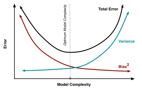
Model Complexity vs. Parsimony

Suppose we have \(p = 30\) covariates (in the true model) and n = 50 observations. We could consider the following two alternatives:

1. We could fit a model using all of the covariates.
   • In this case, \(\widehat\beta\) is unbiased for \(\beta\) (in a linear model fit using OLS). But \(\widehat\beta\) has very high variance.
2. We could fit a model using only the five strongest covariates.
   • In this case, \(\widehat\beta\) will more likely be biased for \(\beta\), but it will have lower variance (compared to the estimate including all covariates)

• Increasing the number of observations sometimes, but not always, helps with the first approach

Source: http://scott.fortmann-roe.com/docs/BiasVariance.html

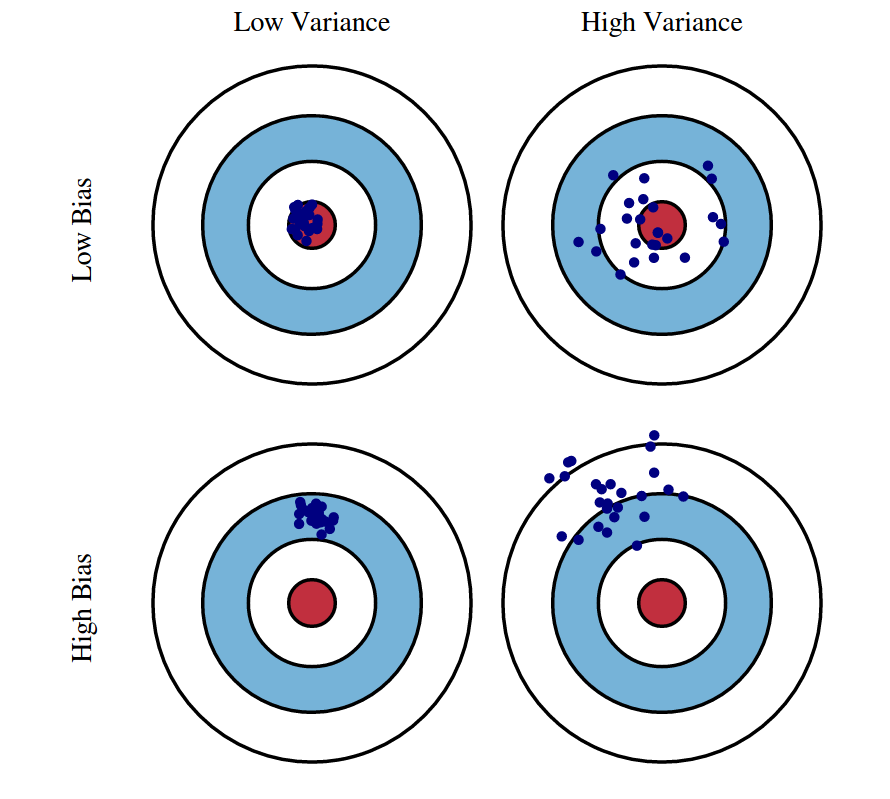
Bias-variance trade off

• Recall mean square error is a function of SSE (sum of squared residuals)

  \[ MSE = \dfrac{1}{n} \sum_{i=1}^{n} \big(Y_i - \widehat{Y}_i \big)^2 = \dfrac{1}{n} SSE \]

• MSE can also be written as a function of the bias and variance

  \[ MSE = \text{bias}\big(\widehat\beta\big)^2 + \text{variance}\big(\widehat\beta\big) \]

• For the same data:

  • More covariates in model: less bias, more variance

  • Less covariates in model: more bias, less variance

• Our goal: find a model with just the right amount of covariates to balance bias and vairance

Source: http://scott.fortmann-roe.com/docs/BiasVariance.html

Model Selection basics (slide adjusted from Jodi Lapidus)

• “Because models always fall far short of the complex reality under study, there are no best or optimal strategies for modeling.”

  • From: Statistical Foundations for Model-Based Adjustments

• Not all statistical texts provide practical advice on model development

  • A lot of resources include methods/code to compare models, but does not include much advice re: selecting which model to ultimately use.
  • Other texts are sparse on details or incorporate simplistic approaches

• Model development strategy should align with research goals

  • Prediction vs. Estimating Association
  • Strategy may depend on study design and data set size

The goals of association vs. prediction

Association / Explanatory / One variable’s effect

• Goal: Understand one variable’s (or a group of variable’s) effect on the response after adjusting for other factors

• Mainly interpret the coefficient of the variable that is the focus of the study

  • Interpreting the coefficients of the other variables is not important, but can help bring context

• Any variables not selected for the final model have still been adjusted for, since they had a chance to be in the model

• Example: How is body mass of a penguin associated with flipper length?

Prediction

• Goal: to calculate the most precise prediction of the response variable

• Interpreting coefficients is not important

• Choose only the variables that are strong predictors of the response variable

  • Excluding irrelevant variables can help reduce widths of the prediction intervals

• Example: What is the flipper length of a penguin with body mass of 3000 g (and all its other characteristics)?

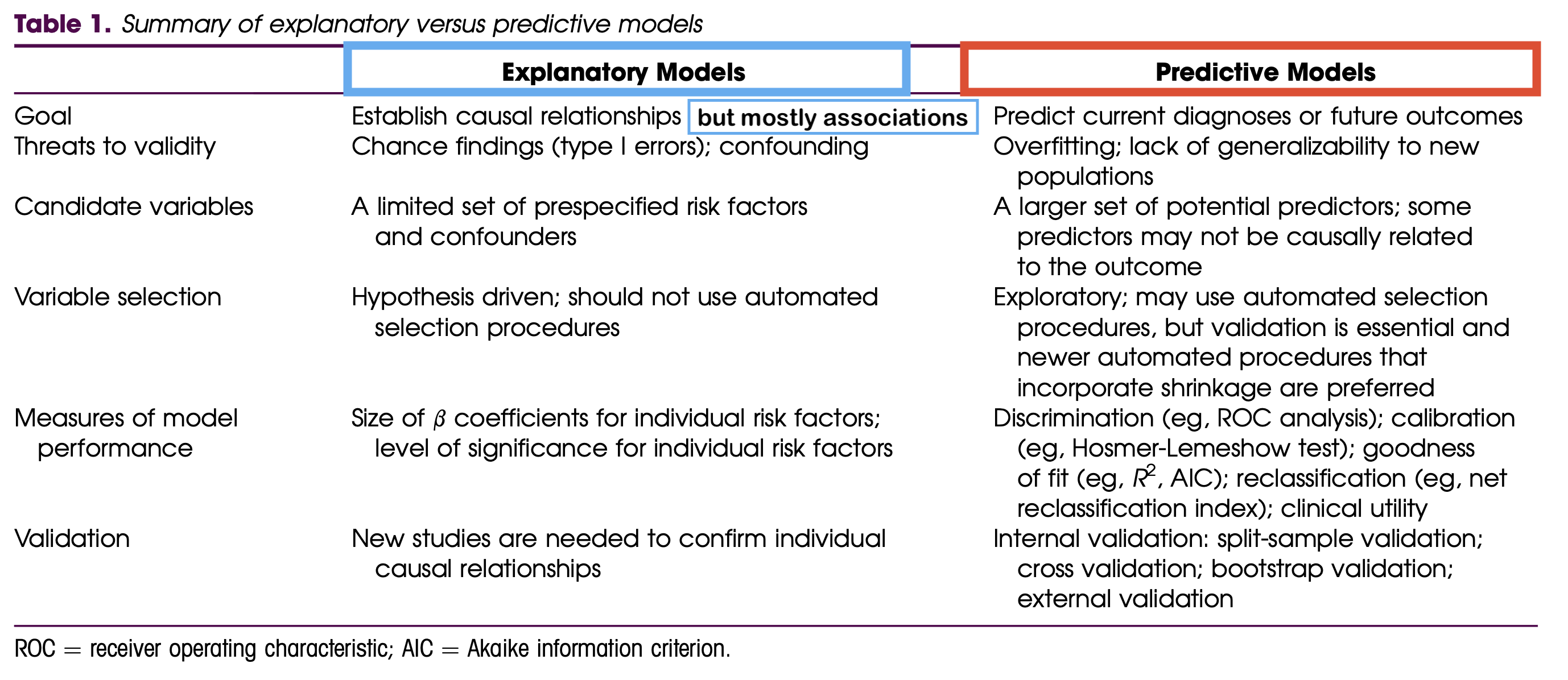
Model building for association vs. prediction

More information on the two analysis goals:

If you ever get the chance, check out Dr. Kristin Sainani’s series on Statistics

Poll Everywhere Question 1

Model selection strategies for continuous outcomes

Association / Explanatory / One variable’s effect

• Selection of potential models is tied more with the research context with some incorporation of prediction scores

• Pre-specification of multivariable model

• Purposeful model selection

  • “Risk factor modeling”

• Change in Estimate (CIE) approaches

  • Will learn in Survival Analysis (BSTA 514)

Prediction

• Selection of potential models is fully dependent on prediction scores

• Automated strategies

  • Stepwise selection (forward/backward)
    • You’ll see these a lot, but they’re not really good methods
  • Best subset
  • Regularization techniques (LASSO, Ridge, Elastic net)

• For categorical outcomes, there are more prediction model selection strategies (will learn more in BSTA 513)

  • Examples: Decision trees, Random forest, Neural networks, K-means

Learning Objectives

1. Understand the motivation for model selection, including bias-variance trade off and alignment of research goals (association vs. prediction)

2. Explain the general process or idea behind different model selection techniques

3. Recognize common model fit statistics and understand what they measure

Pre-specification of multivariable model (slide adapted from Jodi Lapidus)

• In a clinical trial, we often have to write and finalize a statistical analysis plan (SAP) before the trial starts

  • Basically: we completely define the model that we will fit (based on previous work and literature)

 

• If we wish to compare treatment effects adjusted for covariates, all covariates typically specified in advance

  • Example: Comparing effectiveness of 3-drug vs. 2-drug regimen for delaying AIDS onset or death. Covariates such as severity of HIV infection at baseline would have been specified in advance.

  • Variables such as study site, as well as any randomization stratification variables are common covariates.

  • Partly to make sure that we are not adding in variables that make our regimen significant

 

• In these cases, only a limited number of multivariable models are fit and reported

  • Do not perform all the model building steps outlined in Hosmer and Lemeshow texts

Purposeful model selection (slide adapted from Jodi Lapidus)

• Can use this type of model selection for any type of regression

• Careful, well-thought out variable selection process

  • Considers both confounding and interaction, as well as checking model assumptions, fit, etc.

• Often a reasonable strategy, especially in epidemiology and more exploratory clinical studies

  • However, not always appropriate!
  • E.g. clinical trials with model specified in advance. (pre-specified model)

 

• This is the selection process that we will focus on in this class!
  • Next lecture

Change in estimate (CIE) approach (slide adapted from Jodi Lapidus)

• CIE strategies select covariates on the basis of how much their control changes exposure effect estimates

  • Observed change is presumed to measure confounding by the covariate.

• What estimate?

  • Hosmer/Lemeshow (H/L) text suggest using coefficients from the model
  • We typically use the coefficient estimate from the explanatory variable that we are most interested in

• What magnitude change is ”important”?

  • H/L text suggest 10%

• One must choose an effect measure to judge change importance, where “importance” needs to be evaluated along a contextually meaningful scale

• Accurate assessment of confounding may require examining changes from removing entire sets of covariates

  • Add in or eliminate candidate confounders one at time?
  • Add in or eliminate candidate confounders in sets?

Stepwise selection (slide adapted from Adrianna Westbrook)

• This is an incredibly common approach that statisticians use, often because it is an older and more recognized method

  • BUT IT IS ALSO ONE OF THE WORST MODEL SELECTION STRATEGIES!!

• Major disadvantages to stepwise selection:

  • Prone to overfitting
  • Biased estimates
  • Cements the wrong idea that we are looking for our “most significant” covariates

• Predictors/covariates are added or removed one at time if they are below a certain threshold (usually p-value below 0.10 to 0.20)

Stepwise selection: two common approaches

• I will introduce two of the approaches so that you understand the general process if a collaborator ever mentions stepwise selection

• Forward selection:

  • For \(p\) covariates potential covariates, run all simple linear regressions:

    • \(Y= \beta_0 + \beta_1 X_1 + \epsilon\) through \(Y= \beta_0 + \beta_1 X_{p} + \epsilon\)
    • Include the \(X_i\) with the lowest p-value (assuming it is below the threshold)

  • Now run \(Y= \beta_0 + \beta_1 X_i + \beta_2 X_1 + \epsilon\) through \(Y= \beta_0 + \beta_1 X_i + \beta_2 X_{p} + \epsilon\) and enter the next \(X_j\) with the lowest p-value

  • Continue process until no more predictors come back with a p-value below the threshold

• Backward selection:

  • Start with a full model (\(Y= \beta_0 + \beta_1 X_1 + ... + \beta_p X_p + \epsilon\)) and remove predictor with the highest p-value (assuming it is above the threshold)
  • Repeatedly remove the variable with the highest p-value until all remaining variables meet the stopping criteria (are below the threshold)

Best subset (slide adapted from Adrianna Westbrook)

• I don’t see this approach very often

• Quite literally making subsets of the data and using the “best” one

• General steps:

  • Run every possible model fitting 1 to all possible \(p\) predictors/covariates
  • You can limit number of potential predictors
  • \(2^p\) = total number of models where \(p\) = number of predictors
  • You will get the best fitting model within each category (i.e., 1 predictor model, 2 predictor model,…, \(p\) predictor model)
  • Then have to find the best fitting model between the best models from each category

• Major disadvantages to best subset:

  • Does not account for interactions
  • Needs to run a lot of models (takes A LOT of time)

Regularization techniques

• Regularization techniques (LASSO, ridge, elastic net) adds a penalization that shrinks (or regularizes) coefficients down to reduce overfitting
• Maximize likelihood of a model, but includes a penalty for additional covariates

	LASSO (Least About Shrinkage and Selection Operator)	Ridge	Elastic Net
Penalization	L-1 Norm, uses absolute value	L-2 Norm, uses squared value	Best of both worlds, L-1 and L-2 used
Pro’s	Reduces overfitting, will shrink coefficient to zero	Reduces overfitting, handles collinearity, can handle k>n	Reduces overfitting, handles collinearity, handles k>n, shrinks coefficients to zero
Con’s	Cannot handle k>n, doesn’t handle multicollinearity well	Does not shrink coefficients to zero, difficult to interpret	More difficult for R to do than the other two (but not really that bad)

Poll Everywhere Question 2

Learning Objectives

1. Understand the motivation for model selection, including bias-variance trade off and alignment of research goals (association vs. prediction)
2. Explain the general process or idea behind different model selection techniques

3. Recognize common model fit statistics and understand what they measure

Introduction to model fit statistics

• So far we have compared models using the F-test

• The F-test is a great way to compare models that are nested

  • Basically, this means that the “full” model contains all the covariates that the “reduced” model contains
  • The full model will have additional covariates, but the covariates in the reduced is a subset of the covariates in the full

• What if we want to compare models that are not nested?

  • There is a special group of fit statistics that can help us compare models

  • Note: these are sometimes used in the model building process (within one strategy)

    • Helpful if we want to compare selected models across strategies

    • Helpful if we have a few “final” models with different covariates that we want to compare

Common model fit statistics

• The following model fit statistics combine information about the SSE, the number of parameters in the model, and the sample size

• For Mallow’s Cp, AIC, and BIC: smaller values indicate better model fit!

• For Adjusted R-squared: larger values indicate better model fit!

Fit statistic	Equation	R code
R-squared / Adjusted R-squared	\(Adj. R^2 = 1 - \frac{SSE/(n-p-1)}{SSY/(n-1)}\)	Within summary(model_name)
Mallow’s \(C_p\)	\(C_p = \Bigg[ \dfrac{\widehat\sigma^2_p}{\widehat\sigma^2_{max}} - 1 \Bigg](n-p) + p\)	ols_mallows_cp()
Akaike information criterion (AIC)	\(AIC = n\log(SSE) - n \log(n) + 2(p+1)\)	AIC(model_name)
Bayesian information criterion (BIC)	\(BIC = n\log(SSE) - n\log(n) + log(n)\cdot(p+1)\)	BIC(model_name)

 

• We don’t need to know the exact formulas for them!

Common model fit statistics

• There is no hypothesis testing for these fit statistics

  • Only helpful if you are comparing models

  • Works for nested and non-nested models

• Common to report all or some of them

• All of the fit statistics will not necessarily reach a consensus about the best fitting model

  • Each weigh SSE, number of parameters, and number of observations differently

https://www.researchgate.net/figure/Model-Fit-Statistics_tbl1_308844501

Example of a table for model fit statistics

library(olsrr)
model1 = gapm_sub %>% lm(formula = LifeExpectancyYrs ~ FemaleLiteracyRate)
model2 = gapm_sub %>% lm(formula = LifeExpectancyYrs ~ FemaleLiteracyRate + FoodSupplykcPPD)
model3 = gapm_sub %>% lm(formula = LifeExpectancyYrs ~ FemaleLiteracyRate + FoodSupplykcPPD + 
                           income_levels + four_regions)

fit_stats = data.frame(Model = c("Model 1: FLR only", "Model 2: FLR + FS", "Model 3: FLR + FS + Income + WR"), 
                       adj_R_2 = c(summary(model1)$adj.r.squared, summary(model2)$adj.r.squared, 
                                   summary(model3)$adj.r.squared), 
                       Cp = c(ols_mallows_cp(model1, model3), ols_mallows_cp(model2, model3), 
                              ols_mallows_cp(model3, model3)), 
                       AIC = c(AIC(model1), AIC(model2), AIC(model3)), 
                       BIC = c(BIC(model1), BIC(model2), BIC(model3)))

colnames(fit_stats) = c("Model", "Adj. R-squared", "Mallow's Cp", "AIC", "BIC")

fit_stats %>% gt() %>% tab_options(table.font.size = 40) %>% fmt_number(decimals = 3)

Model	Adj. R-squared	Mallow's Cp	AIC	BIC
Model 1: FLR only	0.413	88.126	470.066	476.896
Model 2: FLR + FS	0.550	51.942	451.872	460.979
Model 3: FLR + FS + Income + WR	0.737	9.000	418.724	441.491