Lesson 14: Purposeful model selection
2025-02-26
Regression analysis process

![]()
![]()
Model Selection
Building a model
Selecting variables
Prediction vs interpretation
Comparing potential models
Model Fitting
Find best fit line
Using OLS in this class
Parameter estimation
Categorical covariates
Interactions
Model Evaluation
- Evaluation of model fit
- Testing model assumptions
- Residuals
- Transformations
- Influential points
- Multicollinearity
Model Use (Inference)
- Inference for coefficients
- Hypothesis testing for coefficients
- Inference for expected \(Y\) given \(X\)
- Prediction of new \(Y\) given \(X\)
Pre-step: Exploratory data analysis: Check the data
Get to know the potential values for the data
Categories
Units
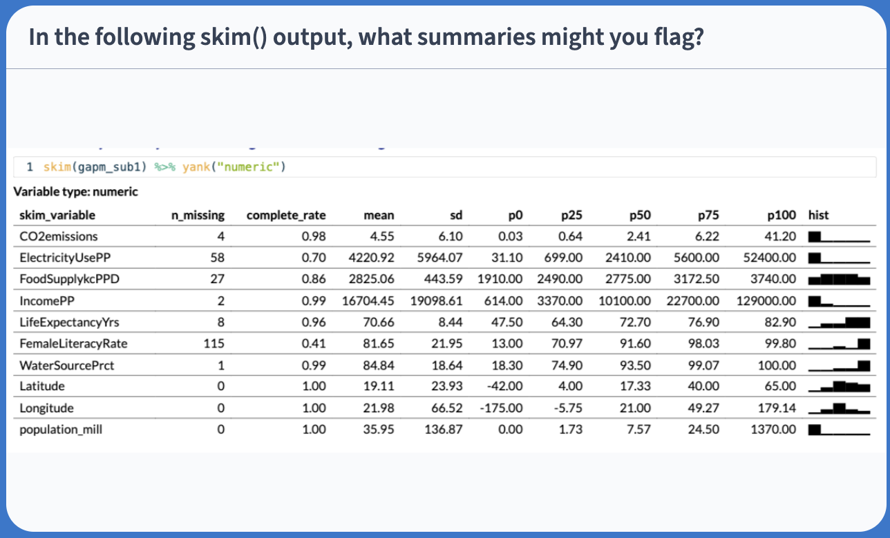
Then make sure the summary of values makes sense
- If minimum or maximum look outside appropriate range
- For example: a negative value for a measurement that is inherently positive (like population or income)
Poll Everywhere Question 1
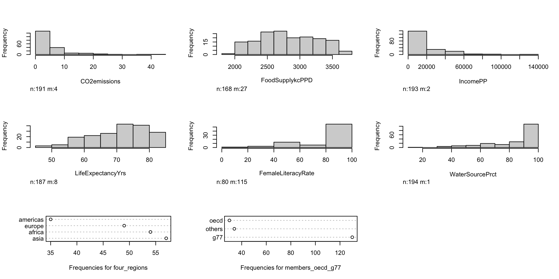
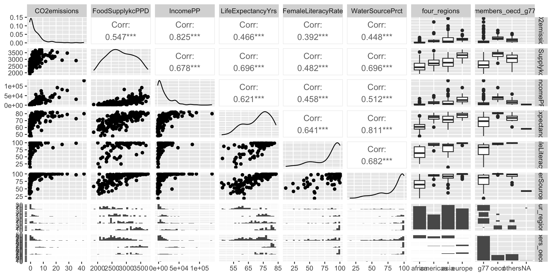
Pre-step: Exploratory data analysis: Study your variables
Pre-step / Step 1 : Explore simple relationships and assumptions
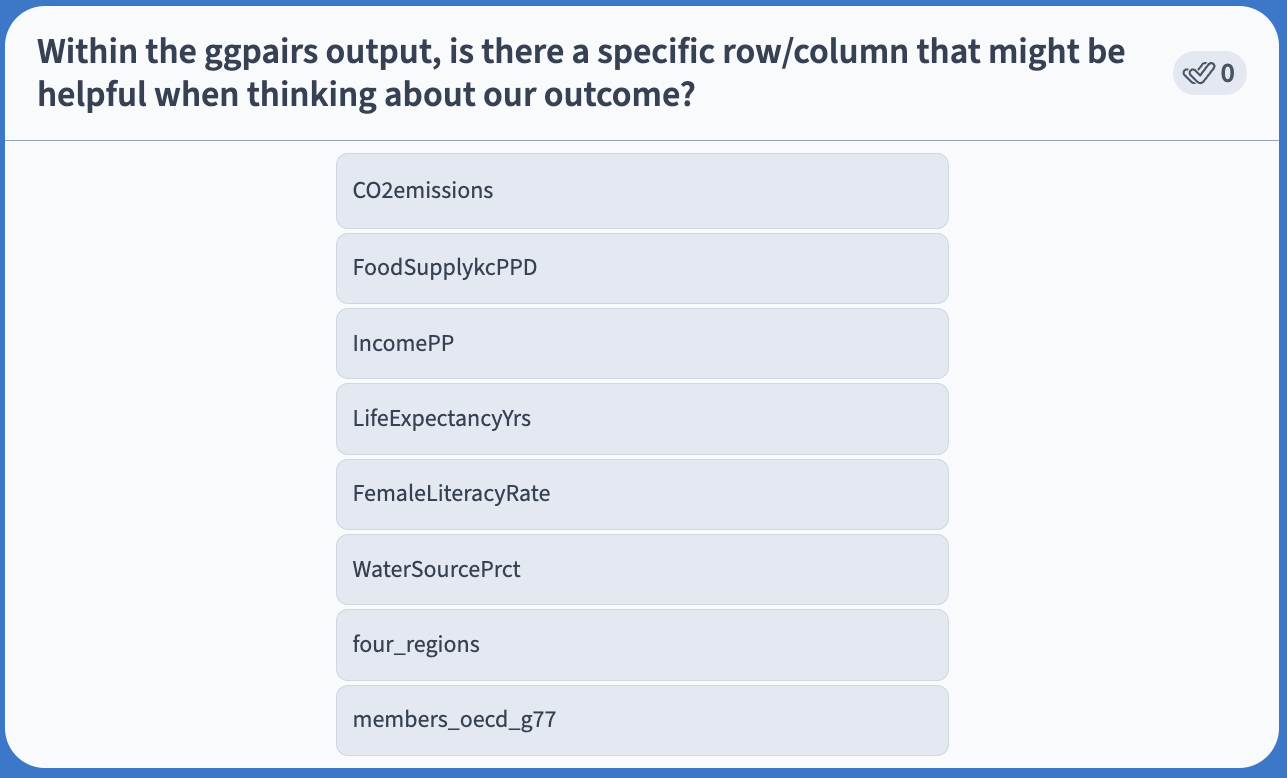
Poll Everywhere Question 3
Step 1: Simple linear regressions / analysis
Let’s think back to our Gapminder dataset
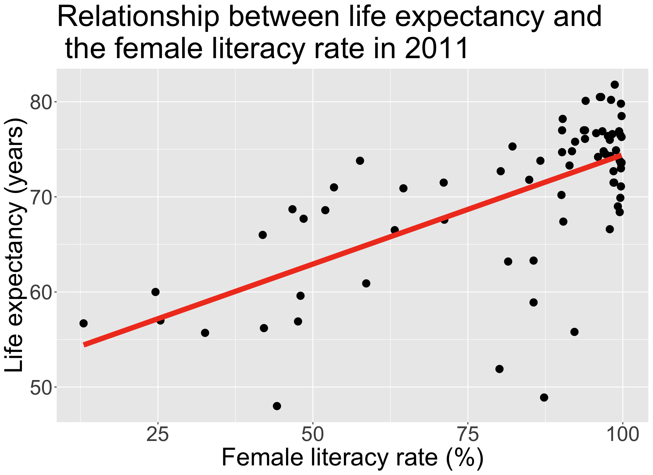
Always good to start with our main relationship: life expectancy vs. female literacy rate
- Throwback to Lesson 3 SLR when we first visualized and ran
lm()for this relationship
- Throwback to Lesson 3 SLR when we first visualized and ran
| term | estimate | std.error | statistic | p.value |
|---|---|---|---|---|
| (Intercept) | 51.438 | 2.739 | 18.782 | 0.000 |
| FemaleLiteracyRate | 0.230 | 0.032 | 7.141 | 0.000 |
Step 1: Simple linear regressions / analysis
- Let’s do this with one other variable before I show you a streamlined version of SLR
Code
ggplot(gapm_sub, aes(x = four_regions, y = LifeExpectancyYrs)) +
  geom_jitter(size = 1, alpha = .6, width = 0.2) +
  stat_summary(fun = mean, geom = "point", size = 8, shape = 18) +
  labs(x = "World region",
       y = "Country life expectancy (years)",
       title = "Life expectancy vs. world region",
       caption = "Diamonds = region averages") +
  theme(axis.title = element_text(size = 20),
        axis.text = element_text(size = 20),
        title = element_text(size = 20))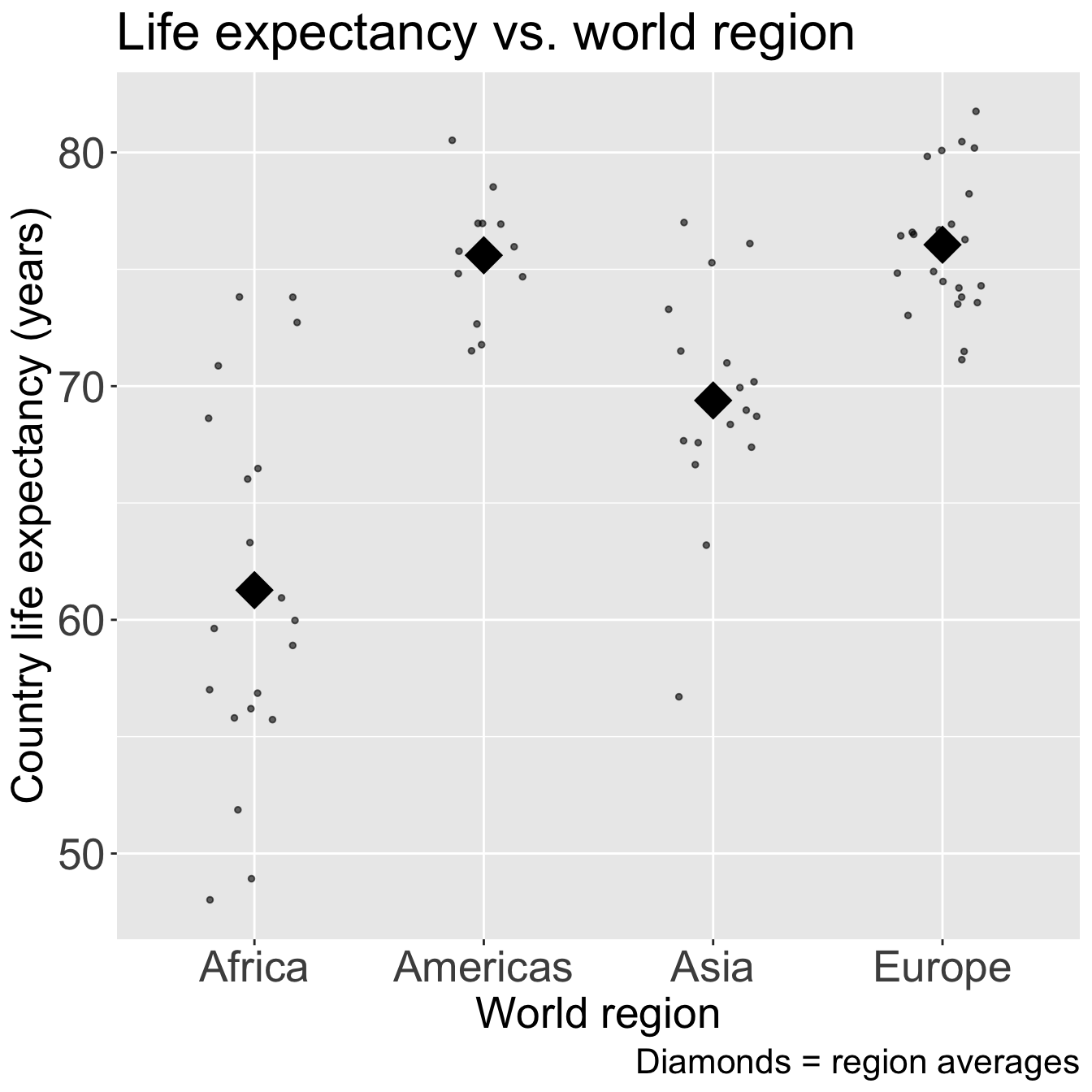
anova(model_WR) %>% tidy() %>% gt() %>%
   tab_options(table.font.size = 40) %>%
fmt_number(decimals = 3)| term | df | sumsq | meansq | statistic | p.value |
|---|---|---|---|---|---|
| four_regions | 3.000 | 2,743.042 | 914.347 | 33.680 | 0.000 |
| Residuals | 68.000 | 1,846.077 | 27.148 | NA | NA |
Recall from Lesson 5 (SLR: More inference + Evaluation):
anova()with one model name will compare the model (model_WR) to the intercept model
Step 4: Assess scale for continuous variables: Smoothed scatterplots
Step 4: Assess scale for continuous variables: Smoothed scatterplots
Take a look at C02, Food Supply, and Income
CO2 = ggplot(data = gapm2, aes(y = LifeExpectancyYrs, x = CO2emissions)) +
  geom_point() +
  geom_smooth(se=F) + labs(x = "CO2 Emissions (kt)", y = "Life Expectancy (yrs)")

FS = ggplot(data = gapm2, aes(y = LifeExpectancyYrs, x = FoodSupplykcPPD)) +
  geom_point() +
  geom_smooth(se=F) + labs(x = "Food Supply (kcal PPD)", y = "Life Expectancy (yrs)")

Income = ggplot(data = gapm2, aes(y = LifeExpectancyYrs, x = IncomePP)) +
  geom_point() +
  geom_smooth(se=F) + labs(x = "Income (GDP per capita)", y = "Life Expectancy (yrs)")

grid.arrange(CO2, FS, Income, nrow=1)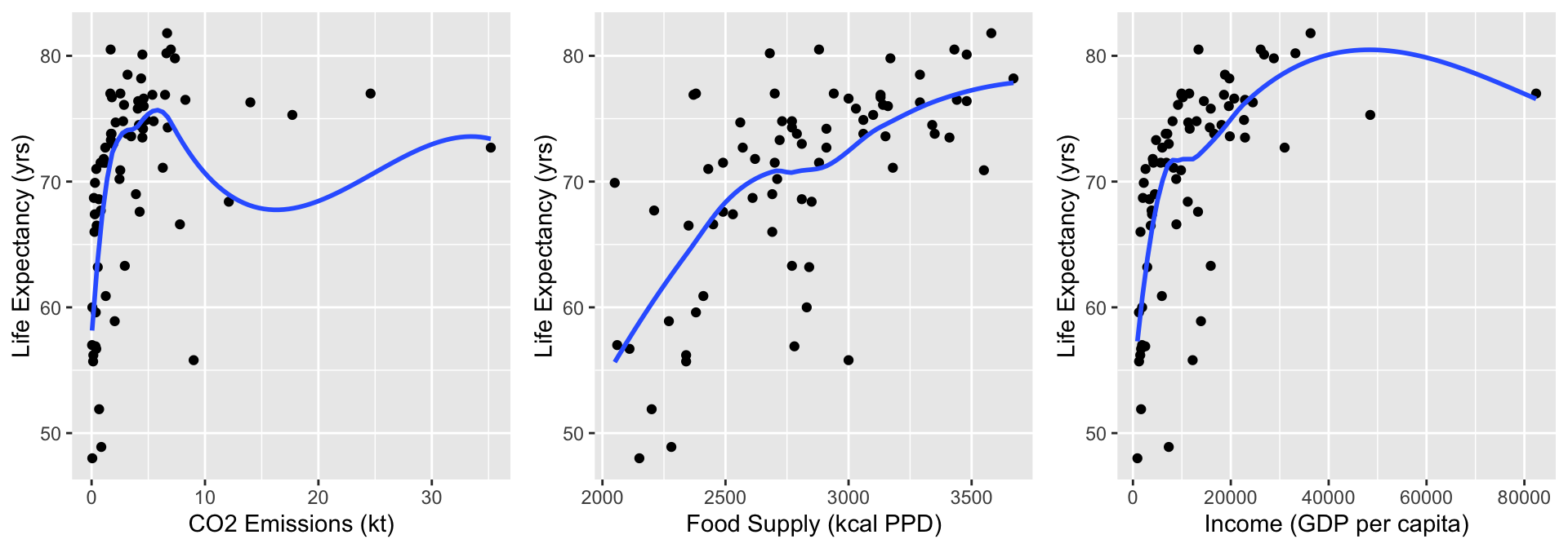
- Food Supply looks admissible
- CO2 Emissions and Income do not look very linear, but I want to zoom into the area of the plots that have most of the data
Step 4: Assess scale for continuous variables: Smoothed scatterplots
Zoom into areas on plots with more data
CO2 = ggplot(data = gapm2, aes(y = LifeExpectancyYrs, x = CO2emissions)) +
  geom_point() + xlim(0,10) +
  geom_smooth(se=F) + labs(x = "CO2 Emissions (kt)", y = "Life Expectancy (yrs)")

FS = ggplot(data = gapm2, aes(y = LifeExpectancyYrs, x = FoodSupplykcPPD)) +
  geom_point() +
  geom_smooth(se=F) + labs(x = "Food Supply (kcal PPD)", y = "Life Expectancy (yrs)")

Income = ggplot(data = gapm2, aes(y = LifeExpectancyYrs, x = IncomePP)) +
  geom_point() + xlim(0,40000) +
  geom_smooth(se=F) + labs(x = "Income (GDP per capita)", y = "Life Expectancy (yrs)")

grid.arrange(CO2, FS, Income, nrow=1)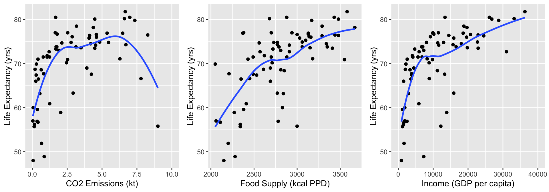
- Food Supply still looks admissible
- CO2 Emissions and Income not linear: will address this!!
Step 4: Approach 1: Categorize continuous variable
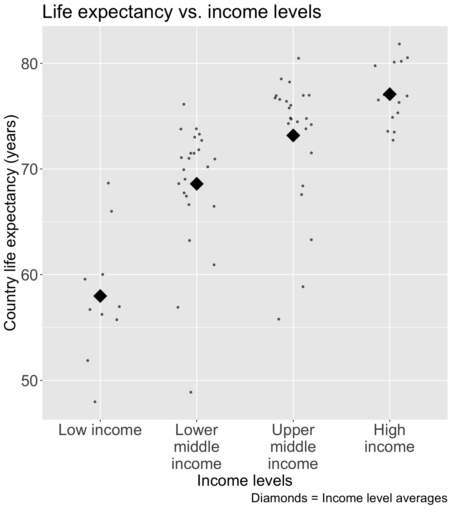
For income, I would use Gapminder’s income level groups
- Discussed in Lesson 10 Categorical Covariates (slide 43)
Experts in the field have developed these income groups
- I think this is best solution for income (that was not meeting linearity as a continuous variable)
Step 4: Approach 1: Categorize continuous variable
Let’s still try it out with CO2 Emissions (kt)
I have plotted the quartile lines of food supply with red lines
Take a look at the quartiles within the scatterplot
vline_coordinates= data.frame(Quantile_Name=names(quantile(gapm2$CO2emissions)),
                          quantile_values=as.numeric(quantile(gapm2$CO2emissions)))

ggplot(data = gapm2, aes(y = LifeExpectancyYrs, x = CO2emissions)) +
  geom_point(size = 3) +
  #geom_smooth(se=F) +
  labs(x = "CO2 Emissions (kt)", y = "Life Expectancy (yrs)") +
  geom_vline(data = vline_coordinates, aes(xintercept = quantile_values),
             color = "red", linetype = "dashed", size = 2) +
    theme(axis.title = element_text(size = 25),
        axis.text = element_text(size = 25),
        title = element_text(size = 25))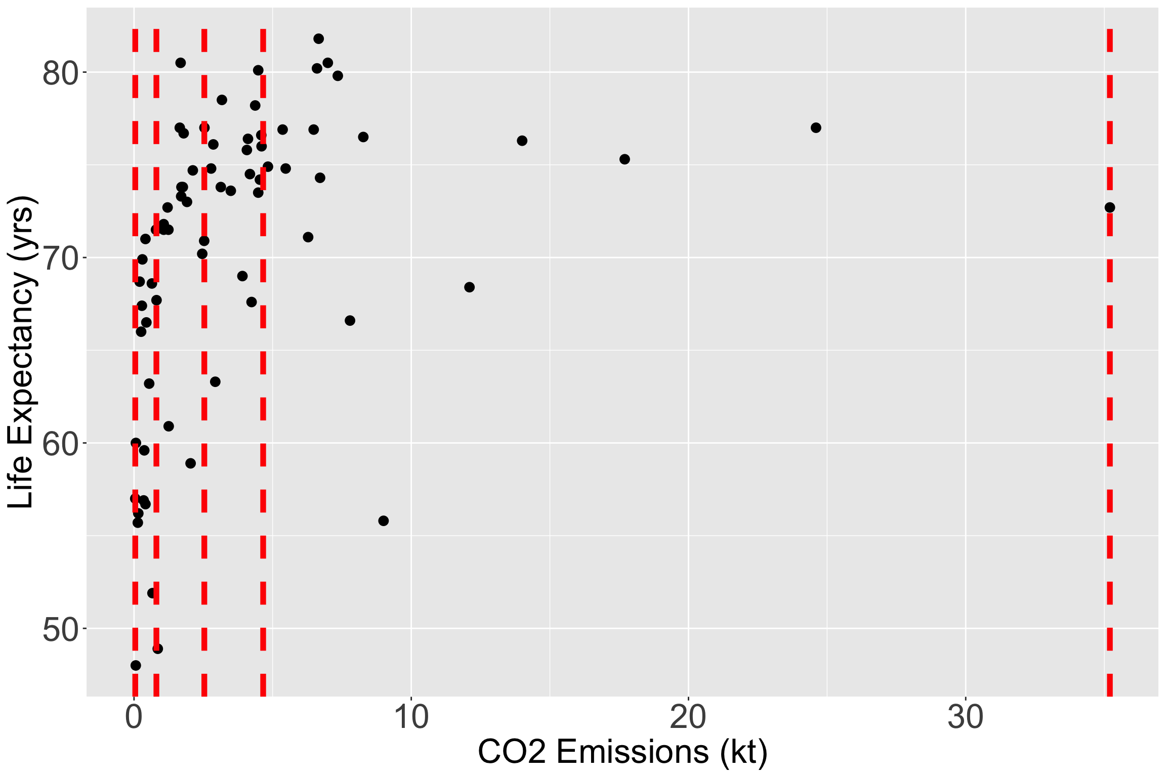
Step 4: Approach 1: Categorize continuous variable
- Let’s make the quartiles for CO2 emissions:
Take a look at the quartile means within the scatterplot
ggplot(data = gapm2, aes(y = LifeExpectancyYrs, x = CO2_q)) +
  # geom_point(size = 3, aes(y = LifeExpectancyYrs, x = CO2emissions)) +
  stat_summary(fun = mean, geom = "point", size = 8, shape = 18) +
  #geom_smooth(se=F) +
  labs(x = "CO2 Emissions (kt)", y = "Life Expectancy (yrs)") +
    theme(axis.title = element_text(size = 25),
        axis.text = element_text(size = 25),
        title = element_text(size = 25))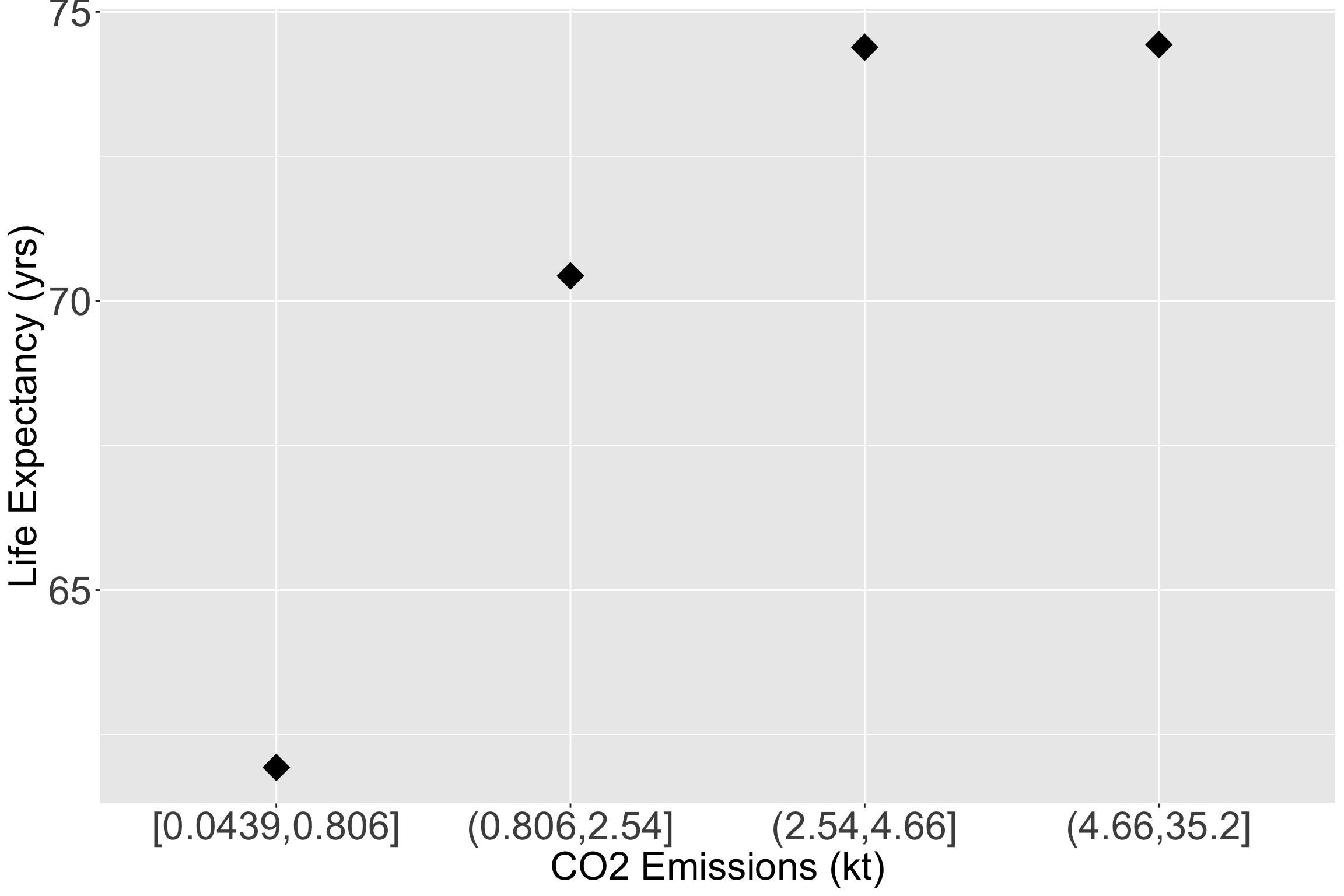
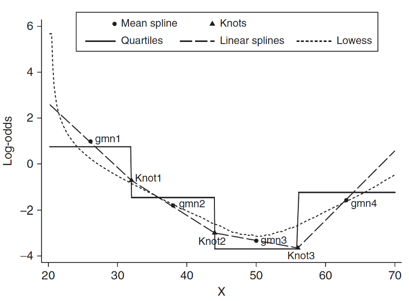
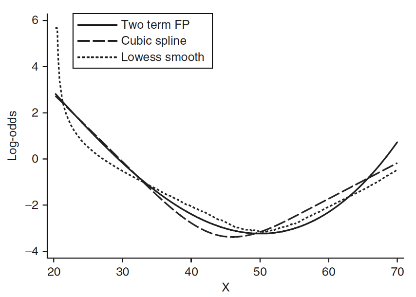
Step 4: Approach 3: Spline functions
- Spline function is to fit a series of smooth curves that joined at specific points (called knots)