Lesson 14: Model Building

With an emphasis on prediction

Nicky Wakim

2026-05-13

Learning Objectives

  1. Understand the place of LASSO regression within association and prediction modeling for binary outcomes.

  2. Understand how penalized regression is a form of model/variable selection.

  3. Set up prediction model building steps and split data into training and testing sets.

  4. Perform LASSO regression on a dataset using R and the general process for classification methods.

Learning Objectives

  1. Understand the place of LASSO regression within association and prediction modeling for binary outcomes.
  1. Understand how penalized regression is a form of model/variable selection.

  2. Set up prediction model building steps and split data into training and testing sets.

  3. Perform LASSO regression on a dataset using R and the general process for classification methods.

Some important definitions

  • Model selection: picking the “best” model from a set of possible models

    • Models will have the same outcome, but typically differ by the covariates that are included, their transformations, and their interactions

    • “Best” model is defined by the research question and by how you want to answer it!


  • Model selection strategies: a process or framework that helps us pick our “best” model

    • These strategies often differ by the approach and criteria used to the determine the “best” model


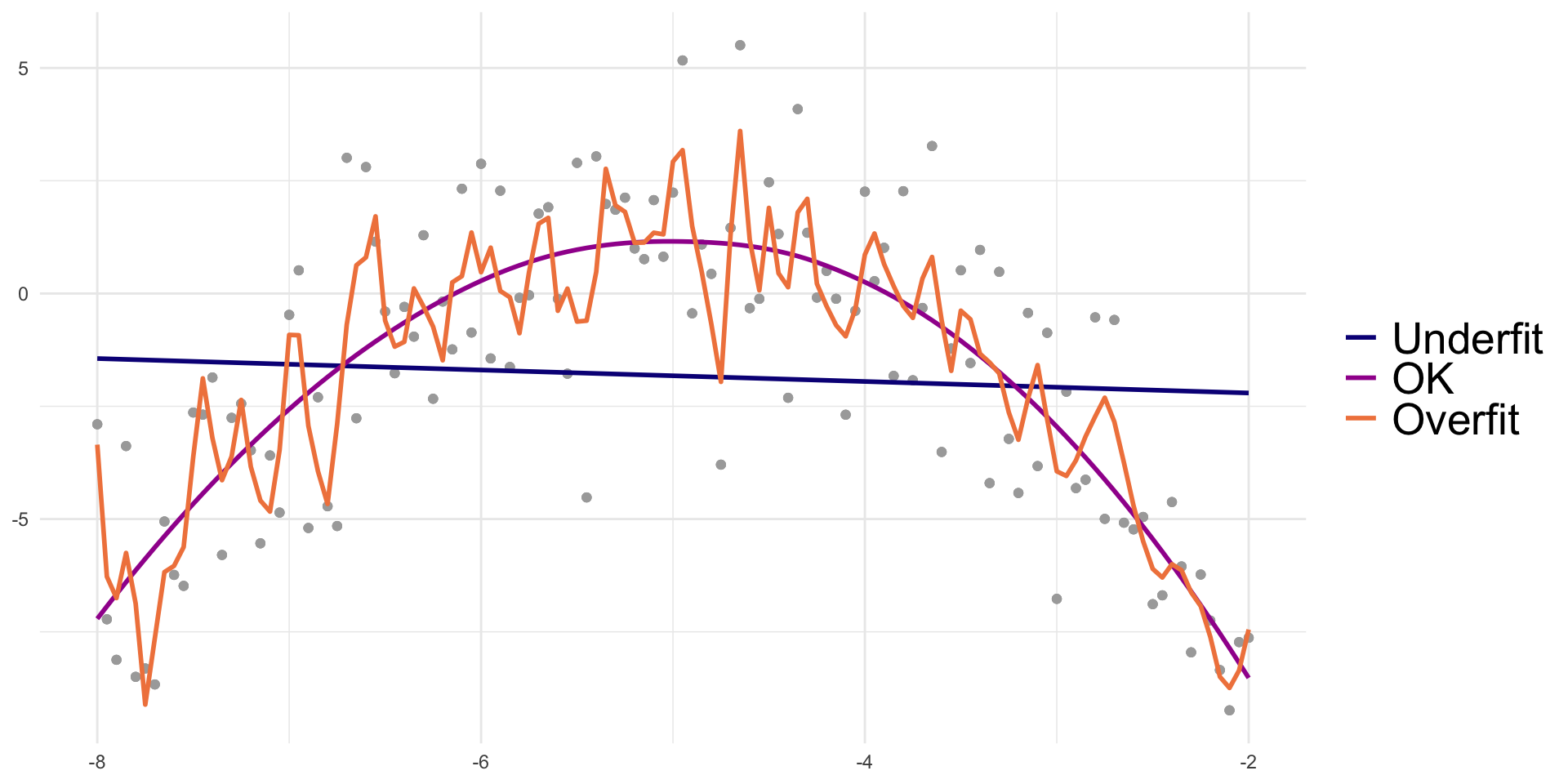
  • Overfitting: result of fitting a model so closely to our particular sample data that it cannot be generalized to other samples (or the population)

Bias-variance trade off

  • Recall from 512/612: MSE can be written as a function of the bias and variance

    \[ MSE = \text{bias}\big(\widehat\beta\big)^2 + \text{variance}\big(\widehat\beta\big) \]

  • No longer use MSE in logistic regression, BUT the idea between the bias and variance trade off holds!

  • For the same data, if our model has…

    • More covariates: less bias, more variance of coef. estimates

      • Potential overfitting: with new data does our model still hold?
    • Less covariates: more bias, less variance of coef. estimates

      • More bias bc more likely that were are not capturing the true underlying relationship with less variables
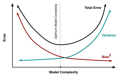
Source: http://scott.fortmann-roe.com/docs/BiasVariance.html

Think of it as a balance between flexibility and stability of our model

Visual of overfitting and underfitting data

From Data Science in a Box:
The goals of association vs. prediction

Association / Explanatory / One variable’s effect

  • Goal: Understand one variable’s (or a group of variable’s) effect on the response after adjusting for other factors
    • Think relationship between variables (outcome and predictor)
  • Mainly interpret odds ratios of the variable that is the focus of the study

  • Research question: How is food insecurity associated with household income?

Prediction

  • Goal: to calculate the most precise prediction of the response variable

  • Interpreting coefficients is not important

  • Choose only the variables that are strong predictors of the response variable

    • Excluding irrelevant variables can help reduce widths of the prediction intervals

  • Research question: How well can we predict food insecurity? What are the biggest conributing factors?

Model selection strategies for categorical outcomes

Association / Explanatory / One variable’s effect

  • Selection of potential models is tied more with the research context with some incorporation of prediction scores

  • Pre-specification of multivariable model

  • Purposeful model selection

    • “Risk factor modeling”
  • Change in Estimate (CIE) approaches

    • Will learn in Time to Event Analysis (BSTA 514)

Prediction

  • Selection of potential models is fully dependent on prediction scores

  • Logistic regression with more refined model selection
    • Regularization techniques (LASSO, Ridge, Elastic net)
  • Machine learning realm
    • Decision trees, random forest, k-nearest neighbors, Neural networks

Before I move on…

  • We CAN use purposeful selection from last quarter in any type of generalized linear model (GLM)

    • This includes logistic regression!


  • The best documented information on purposeful selection is in the Hosmer-Lemeshow textbook on logistic regression


  • I will not discuss purposeful selection in this lesson

    • Be aware that this is a tool that you can use in any regression!
    • You can follow my process for linear regression in Lesson 14 in BSTA 512/612

Okay, so prediction of categorical outcomes

  • Classification: process of predicting categorical responses/outcomes

    • Assigning a category outcome based on an observation’s predictors


  • Note: we’ve already done a lot of work around predicting probabilities within logistic regression

    • Can we take those predicted probabilities one step further to predict the binary outcome??


  • Common classification models (good site on brief explanation of each)

    • Logistic regression
    • Naive Bayes
    • k-Nearest Neighbor (KNN)
    • Decision Trees
    • Support Vector Machines (SVMs)
    • Neural Networks

Logistic regression can be a classification model

  • But to be a good classifier, our logistic regression model needs to…
    • be built a certain way
    • have good potential predictors


  • Prediction depends on type of variable/model selection!

    • This is when it can become machine learning


  • So the big question is: how do we select this model??

    • Regularized techniques, aka penalized regression

Poll Everywhere Question 1

Learning Objectives

  1. Understand the place of LASSO regression within association and prediction modeling for binary outcomes.
  1. Understand how penalized regression is a form of model/variable selection.
  1. Set up prediction model building steps and split data into training and testing sets.

  2. Perform LASSO regression on a dataset using R and the general process for classification methods.

Penalized regression

  • Basic idea: We are running regression, but now we want to incentivize our model to have less predictors

    • Include a penalty to discourage too many predictors in the model


  • Also known as shrinkage or regularization methods
    • “Shrinks” some coefficient estimates to 0


  • Penalty will reduce coefficient values to zero (or close to zero) if the predictor does not contribute much information to predicting our outcome


  • We need a tuning parameter that determines the amount of shrinkage called lambda/\(\lambda\)

    • How much do we want to penalize additional predictors?

Poll Everywhere Question 2

Three types of penalized regression

Main difference is the type of penalty used

Ridge regression

  • Penalty called L2 norm, uses squared values

  • Pros

    • Reduces overfitting
    • Handles \(p>n\)
    • Handles collinearity
  • Cons

    • Does not shrink coefficients to 0
    • Difficult to interpret

Lasso regression

  • Penalty called L1 norm, uses absolute values


  • Pros
    • Reduces overfitting
    • Shrinks coefficients to 0
  • Cons
    • Cannot handle \(p>n\)
    • Does not handle multicollinearity well

Elastic net regression

  • L1 and L2 used, best of both worlds

  • Pros

    • Reduces overfitting
    • Handles \(p>n\)
    • Handles collinearity
    • Shrinks coefficients to 0
  • Cons

    • More difficult to do than other two

The glmnet() and cv.glmnet() functions

  • We are familiar with glm() for fitting generalized linear models


  • For penalized regression, we use glmnet() and cv.glmnet()
    • Can fit many types of outcomes (binary, continuous, count, etc.)
    • Can fit Lasso, Ridge, and Elastic net regression
    • Can include interactions and transformations of predictors
    • Input and output of the function are a little rigid (not very tidyverse compliant)


  • Difference between the two functions:
    • glmnet() fits the model for a sequence of lambda values
    • cv.glmnet() performs cross-validation to find the optimal lambda

Learning Objectives

  1. Understand the place of LASSO regression within association and prediction modeling for binary outcomes.

  2. Understand how penalized regression is a form of model/variable selection.

  1. Set up prediction model building steps and split data into training and testing sets.
  1. Perform LASSO regression on a dataset using R and the general process for classification methods.

Overview of predicton model building steps

  1. Split data into training and testing datasets


  1. Build classification model using training set

    • This is where we will use penalized regression!


  1. Measure predictive accuracy on testing set

Example to be used: GLOW Study

  • From GLOW (Global Longitudinal Study of Osteoporosis in Women) study


  • Outcome variable: any fracture in the first year of follow up (FRACTURE: 0 or 1)


  • Risk factor/variable of interest: history of prior fracture (PRIORFRAC: 0 or 1)

  • Potential confounder or effect modifier: age (AGE, a continuous variable)

    • Center age will be used! We will center around the rounded mean age of 69 years old


  • Crossed out because we are no longer attached to specific predictors and their association with fracture

    • Focused on predicting fracture with whatever variables we can!

Let’s look at our data

glimpse(glow1)
Rows: 500
Columns: 16
$ sub_id    <int> 1, 2, 3, 4, 5, 6, 7, 8, 9, 10, 11, 12, 1…
$ site_id   <int> 1, 4, 6, 6, 1, 5, 5, 1, 1, 4, 6, 1, 6, 1…
$ phy_id    <int> 14, 284, 305, 309, 37, 299, 302, 36, 8, …
$ priorfrac <fct> No, No, Yes, No, No, Yes, No, Yes, Yes, …
$ age       <int> 62, 65, 88, 82, 61, 67, 84, 82, 86, 58, …
$ weight    <dbl> 70.3, 87.1, 50.8, 62.1, 68.0, 68.0, 50.8…
$ height    <int> 158, 160, 157, 160, 152, 161, 150, 153, …
$ bmi       <dbl> 28.16055, 34.02344, 20.60936, 24.25781, …
$ premeno   <fct> No, No, No, No, No, No, No, No, No, No, …
$ momfrac   <fct> No, No, Yes, No, No, No, No, No, No, No,…
$ armassist <fct> No, No, Yes, No, No, No, No, No, No, No,…
$ smoke     <fct> No, No, No, No, No, Yes, No, No, No, No,…
$ raterisk  <fct> Same, Same, Less, Less, Same, Same, Less…
$ fracscore <int> 1, 2, 11, 5, 1, 4, 6, 7, 7, 0, 4, 3, 1, …
$ fracture  <fct> No, No, No, No, No, No, No, No, No, No, …
$ age_c     <dbl> -7, -4, 19, 13, -8, -2, 15, 13, 17, -11,…

Step 1: Splitting data

  • Training: act of creating our prediction model based on our observed data

    • Supervised: Means we keep information on our outcome while training


  • Testing: act of measuring the predictive accuracy of our model by trying it out on new data


  • When we use data to create a prediction model, we want to test our prediction model on new data

    • Helps make sure prediction model can be applied to other data outside of the data that was used to create it!


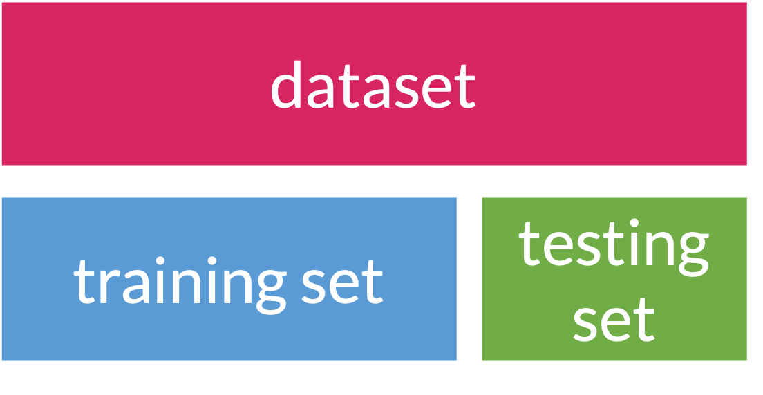
  • So an important first step in prediction modeling is to split our data into a training set and a testing set!
 

Step 1: Splitting data

Training set

  • Sandbox for model building
  • Spend most of your time using the training set to develop the model
  • Majority of the data (usually 80%)

Testing set

  • Held in reserve to determine efficacy of one or two chosen models
  • Critical to look at it once at the end, otherwise it becomes part of the modeling process
  • Remainder of the data (usually 20%)


Poll Everywhere Question 3

Step 1: Splitting data

  • When splitting data, we need to be conscious of the proportions of our outcomes

    • Is there imbalance within our outcome?

    • We want to randomly select observations but make sure the proportions of No and Yes stay the same

    • We stratify by the outcome, meaning we pick Yes’s and No’s separately for the training set
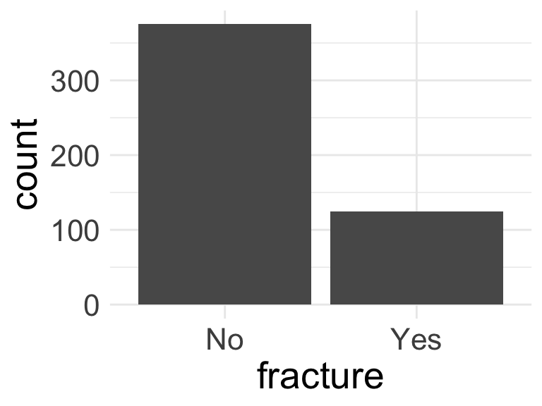
ggplot(glow1, aes(x = fracture)) + geom_bar()

  • Side note: I took out some variables
glow = glow1 %>%
    dplyr::select(-sub_id, -site_id, -phy_id, -age, -bmi, -weight, -fracscore)

Step 1: Splitting data

  • From package rsample within tidyverse, we can use initial_split() to create training and testing data

    • Use strata to stratify by fracture
    • Use prop to set the proportion of training data
glow_split = initial_split(glow, strata = fracture, prop = 0.8)
glow_split
<Training/Testing/Total>
<400/100/500>
  • Then we can pull the training and testing data into their own datasets
glow_train = training(glow_split)
glow_test = testing(glow_split)

Step 1: Splitting data: peek at the split

glimpse(glow_train)
Rows: 400
Columns: 9
$ priorfrac <fct> No, No, Yes, No, No, Yes, No, Yes, Yes, No, No, No, No, No, …
$ height    <int> 158, 160, 157, 160, 152, 161, 150, 153, 156, 166, 153, 160, …
$ premeno   <fct> No, No, No, No, No, No, No, No, No, No, No, Yes, No, No, No,…
$ momfrac   <fct> No, No, Yes, No, No, No, No, No, No, No, Yes, No, No, No, No…
$ armassist <fct> No, No, Yes, No, No, No, No, No, No, No, No, No, Yes, No, No…
$ smoke     <fct> No, No, No, No, No, Yes, No, No, No, No, Yes, No, No, No, No…
$ raterisk  <fct> Same, Same, Less, Less, Same, Same, Less, Same, Same, Less, …
$ fracture  <fct> No, No, No, No, No, No, No, No, No, No, No, No, No, No, No, …
$ age_c     <dbl> -7, -4, 19, 13, -8, -2, 15, 13, 17, -11, -2, -5, -1, -2, 0, …
glimpse(glow_test)
Rows: 100
Columns: 9
$ priorfrac <fct> No, No, No, No, No, No, No, Yes, Yes, No, No, No, No, No, No…
$ height    <int> 167, 162, 165, 170, 154, 160, 171, 142, 152, 166, 154, 163, …
$ premeno   <fct> No, No, No, Yes, Yes, No, Yes, Yes, No, No, No, No, Yes, No,…
$ momfrac   <fct> No, No, No, Yes, No, No, No, Yes, No, No, No, No, Yes, No, N…
$ armassist <fct> Yes, No, Yes, No, Yes, Yes, No, No, No, No, No, No, Yes, No,…
$ smoke     <fct> Yes, Yes, No, No, No, No, No, No, No, No, No, No, Yes, No, N…
$ raterisk  <fct> Same, Less, Less, Same, Same, Less, Same, Same, Same, Same, …
$ fracture  <fct> No, No, No, No, No, No, No, No, No, No, No, No, No, No, No, …
$ age_c     <dbl> -13, -10, 3, 0, 6, -3, -5, 1, 17, -11, -6, -10, -10, 0, -12,…

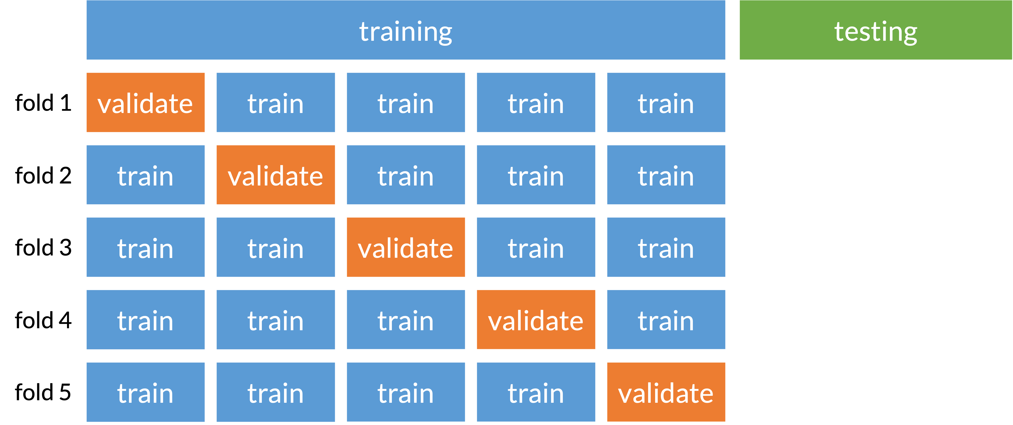
Cross-validation (specifically k-fold)

  • Prevents overfitting to one set of training data

  • Split training set into folds that train and validate model selection

  • We can train and validate several times within the training set

Learning Objectives

  1. Understand the place of LASSO regression within association and prediction modeling for binary outcomes.

  2. Understand how penalized regression is a form of model/variable selection.

  3. Set up prediction model building steps and split data into training and testing sets.

  1. Perform LASSO regression on a dataset using R and the general process for classification methods.

Unfortunately… cv.glmnet() needs a specific input for the data

y_train = as.numeric(glow_train$fracture) - 1 # glmnet needs numeric outcome
# x_train = glow_train %>% select(-fracture) %>% as.matrix() 
f = as.formula(fracture ~ .) 
f
fracture ~ .
x_train = model.matrix(f, data = glow_train)[, -1]
glimpse(x_train)
 num [1:400, 1:9] 0 0 1 0 0 1 0 1 1 0 ...
 - attr(*, "dimnames")=List of 2
  ..$ : chr [1:400] "1" "2" "3" "4" ...
  ..$ : chr [1:9] "priorfracYes" "height" "premenoYes" "momfracYes" ...

Overview of predicton model building steps

  1. Split data into training and testing datasets


  1. Build classification model using training set

    • This is where we will use penalized regression!


  1. Measure predictive accuracy on testing set

Step 2: Fit LASSO penalized logistic regression model

  • Using Lasso penalized regression!

  • We can simply set up a penalized regression model

library(glmnet)
glow_fit <- cv.glmnet(
  y = y_train, 
  x = x_train, 
  family = "binomial", 
  alpha = 1, # 1 for LASSO 
  thresh = 1e-12
  )
  • cv.glmnet uses cross validation and finds the best penalty (lambda)

  • alpha option let’s us pick the penalty

    • alpha = 0 for Ridge regression
    • alpha = 1 for Lasso regression
    • 0 < alpha < 1 for Elastic net regression

Step 2: Fit LASSO: Coefficient estimates (kinda)

  • We can look at the coefficient estimates of the model at the best lambda
  • “Best lambda” is lambda.min in the output of cv.glmnet()
beta = coef(glow_fit, s = "lambda.min", x = x_train, y = y_train)
beta
10 x 1 sparse Matrix of class "dgCMatrix"
                 lambda.min
(Intercept)      3.87740705
priorfracYes     0.76550436
height          -0.03648382
premenoYes       0.28439319
momfracYes       0.79923255
armassistYes     0.26670345
smokeYes        -0.23118903
rateriskSame     0.41350772
rateriskGreater  0.64369667
age_c            0.03397730
lambda = glow_fit$lambda.min
lambda
[1] 0.00198163

Step 2: Fit LASSO: Main effects: Identify variables

library(vip)  
vi(glow_fit, lambda = glow_fit$lambda.min)
# A tibble: 9 × 3
  Variable        Importance Sign 
  <chr>                <dbl> <chr>
1 momfracYes          0.799  POS  
2 priorfracYes        0.766  POS  
3 rateriskGreater     0.644  POS  
4 rateriskSame        0.414  POS  
5 premenoYes          0.284  POS  
6 armassistYes        0.267  POS  
7 smokeYes            0.231  NEG  
8 height              0.0365 NEG  
9 age_c               0.0340 POS  

Looks like nothing is removed! (Importance would be 0)
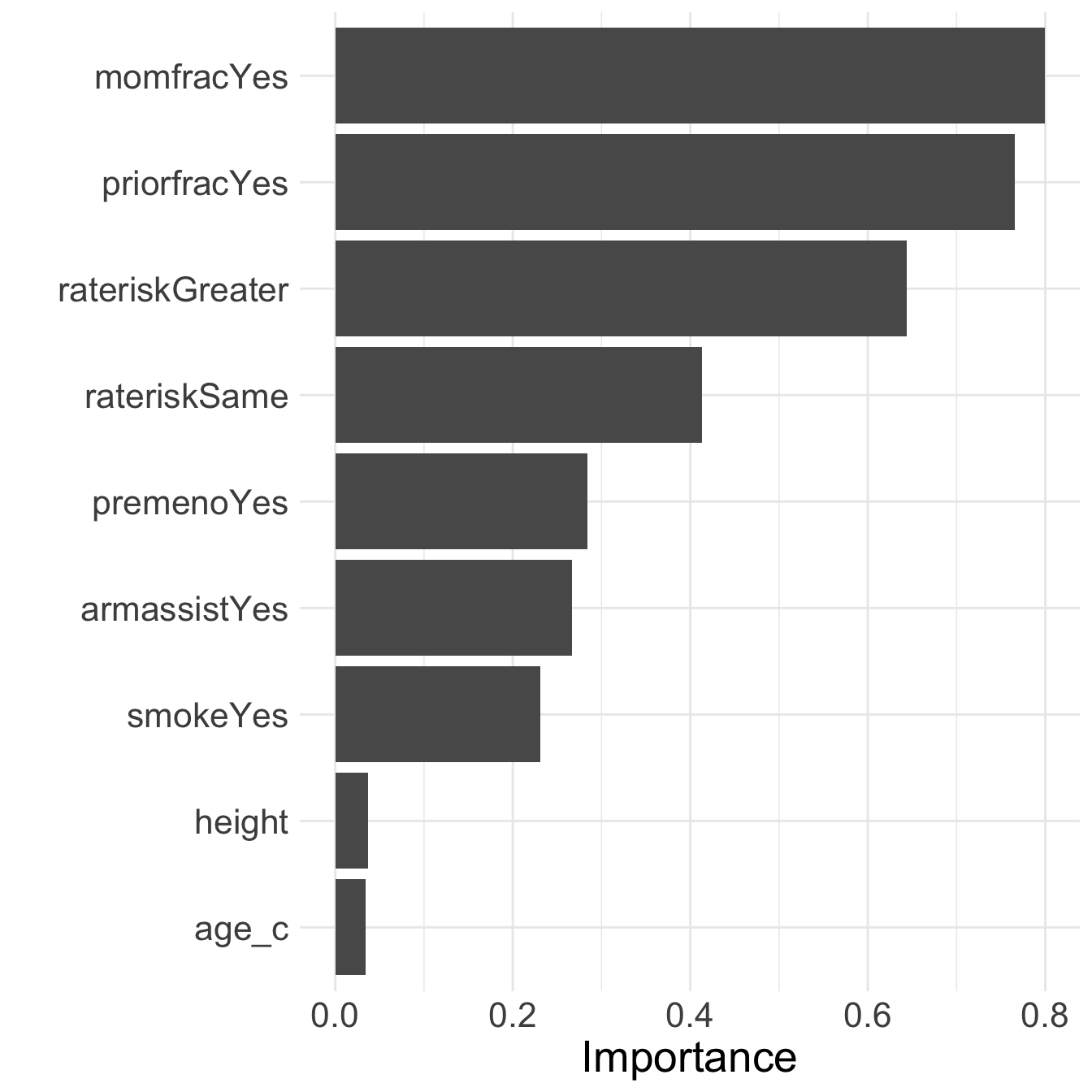
vip(glow_fit, 
    lambda = glow_fit$lambda.min, 
    num_features = 20) + 
  theme(text = element_text(size=20))

STOP!

  • Going to run another model!
  • Just wanted to demonstrate the process with an set of main effects
  • NOW we will include interactions in our model
    • More typical in prediction

Step 2: Fit LASSO: Main effects + interactions

  • Typically, we want to include interactions in our prediction model
f = as.formula(fracture ~ .^2) # formula for main effects and interactions
x_train_int = model.matrix(f, data = glow_train)[, -1] 
glow_fit_int <- cv.glmnet(
  y = y_train, 
  x = x_train_int, 
  family = "binomial", 
  alpha = 1, 
  thresh = 1e-12
  )

Step 2: Fit LASSO interaction model: Coefficient estimates (kinda)

beta_int = coef(glow_fit_int, s = "lambda.min", exact = TRUE, x = x_train, y = y_train)
lambda_int = glow_fit_int$lambda.min
lambda_int
[1] 0.0202826
beta_int
45 x 1 sparse Matrix of class "dgCMatrix"
                                lambda.min
(Intercept)                   2.0850976952
priorfracYes                  0.4943898067
height                       -0.0225868202
premenoYes                    .           
momfracYes                    .           
armassistYes                  .           
smokeYes                      .           
rateriskSame                  .           
rateriskGreater               .           
age_c                         .           
priorfracYes:height           .           
priorfracYes:premenoYes       .           
priorfracYes:momfracYes       .           
priorfracYes:armassistYes     0.3544339464
priorfracYes:smokeYes         .           
priorfracYes:rateriskSame     .           
priorfracYes:rateriskGreater  .           
priorfracYes:age_c            .           
height:premenoYes             .           
height:momfracYes             0.0004091542
height:armassistYes           .           
height:smokeYes               .           
height:rateriskSame           .           
height:rateriskGreater        0.0016221169
height:age_c                  0.0001517309
premenoYes:momfracYes         .           
premenoYes:armassistYes       .           
premenoYes:smokeYes           .           
premenoYes:rateriskSame       .           
premenoYes:rateriskGreater    0.4755109044
premenoYes:age_c              .           
momfracYes:armassistYes       .           
momfracYes:smokeYes           .           
momfracYes:rateriskSame       1.1275503167
momfracYes:rateriskGreater    0.1980126090
momfracYes:age_c              .           
armassistYes:smokeYes         .           
armassistYes:rateriskSame     0.2851098186
armassistYes:rateriskGreater  .           
armassistYes:age_c            .           
smokeYes:rateriskSame         .           
smokeYes:rateriskGreater      .           
smokeYes:age_c                0.0027159535
rateriskSame:age_c            .           
rateriskGreater:age_c         .           

Step 2: Fit LASSO interaction model: Variable importance

vi(glow_fit_int, 
   lambda = lambda_int)
# A tibble: 44 × 3
   Variable                   Importance Sign 
   <chr>                           <dbl> <chr>
 1 momfracYes:rateriskSame      1.13     POS  
 2 priorfracYes                 0.494    POS  
 3 premenoYes:rateriskGreater   0.476    POS  
 4 priorfracYes:armassistYes    0.354    POS  
 5 armassistYes:rateriskSame    0.285    POS  
 6 momfracYes:rateriskGreater   0.198    POS  
 7 height                       0.0226   NEG  
 8 smokeYes:age_c               0.00272  POS  
 9 height:rateriskGreater       0.00162  POS  
10 height:momfracYes            0.000409 POS  
# ℹ 34 more rows
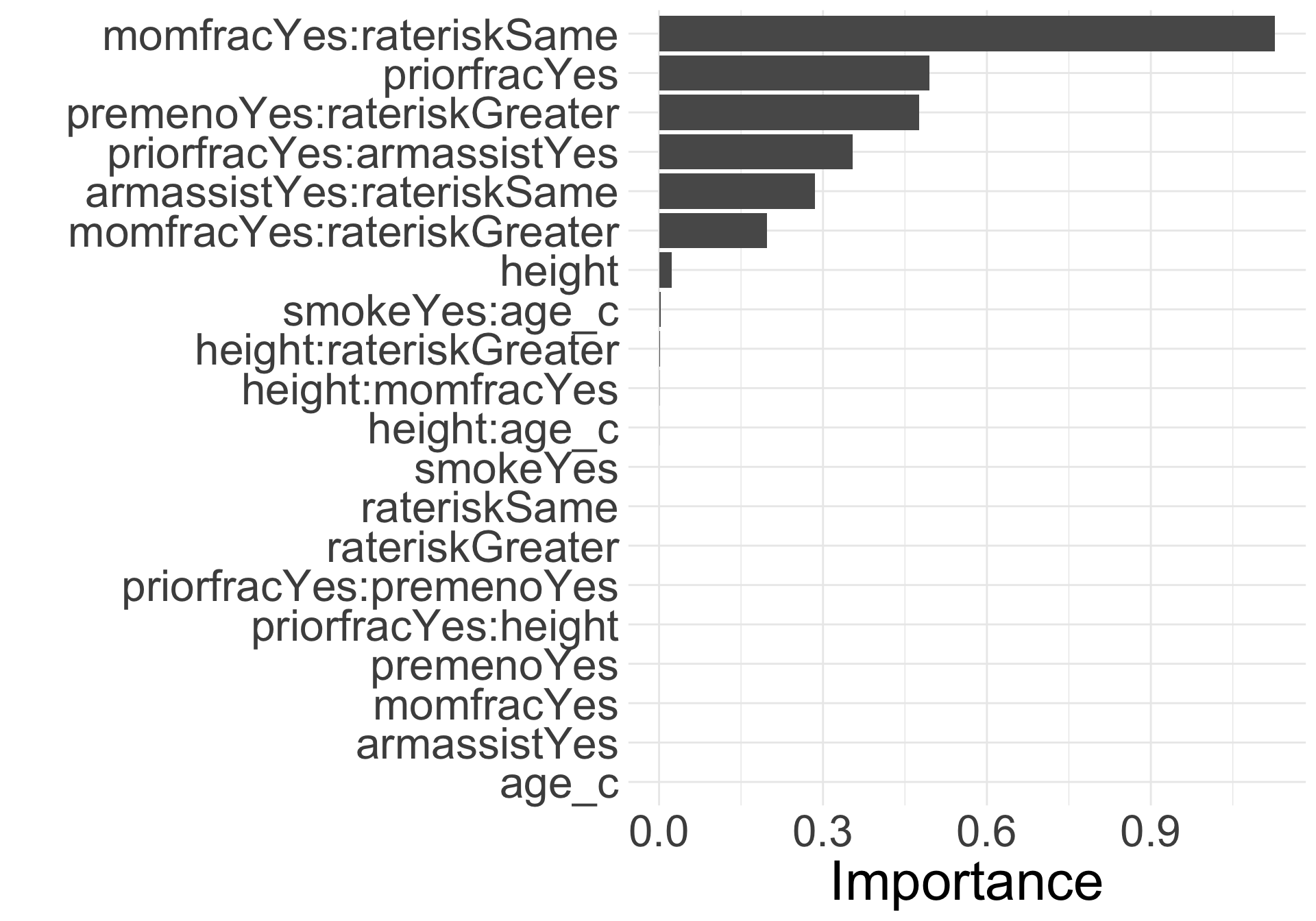
vip(glow_fit_int, 
    lambda =lambda_int, 
    num_features = 20) + 
  theme(text = element_text(size=30))

Step 2: Fit LASSO interaction model: Coefficient estimates (for real)

  • Very specific way we can extract the exact coefficient estimates
  • This uses the values in beta_int to calculate coefficient estimates conditional on fact that those variables were selected
library(selectiveInference)
out = fixedLassoInf(
  x_train_int, 
  y_train, 
  beta_int, 
  lambda_int, 
  family="binomial"
  )

Step 2: Fit LASSO interaction model: Coefficient estimates (for real)

out

Call:
fixedLassoInf(x = x_train_int, y = y_train, beta = beta_int, 
    lambda = lambda_int, family = "binomial")

Testing results at lambda = 0.020, with alpha = 0.100

 Var   Coef Z-score P-value LowConfPt UpConfPt LowTailArea UpTailArea
   1  0.647   1.840   0.220    -0.750    1.568       0.049      0.050
   2 -0.044  -2.173   0.347    -0.073    0.092       0.050      0.050
  13  0.311   0.686   0.311    -1.427    2.970       0.050      0.050
  19 -0.002  -0.303   0.244    -0.211    0.056       0.050      0.050
  23  0.003   1.456   0.294    -0.007    0.012       0.050      0.050
  24  0.000   1.985   0.025     0.000    0.002       0.050      0.050
  29  0.786   1.642   0.194    -0.757    1.695       0.049      0.049
  33  1.972   1.967   0.191    -7.231   34.991       0.050      0.050
  34  0.888   0.881   0.286   -12.816   34.850       0.050      0.050
  37  0.715   1.919   0.364    -1.632    1.335       0.050      0.049
  42  0.052   0.955   0.929    -3.202    0.033       0.050      0.050

Note: coefficients shown are full regression coefficients

We can “tidy” the output and transform to ORs

  • Use tibble to make tidy and take exponential of coefficients
lasso_inference_df <- tibble(
  term      = names(out$vars),
  estimate  = exp(out$coef0),
  std.error = out$sd,
  statistic = out$z,
  p.value   = out$pv,
  conf.low  = exp(out$ci[,1]),
  conf.high = exp(out$ci[,2])
)

We can “tidy” the output and transform to ORs

lasso_inference_df
# A tibble: 11 × 7
   term                  estimate std.error statistic p.value conf.low conf.high
   <chr>                    <dbl>     <dbl>     <dbl>   <dbl>    <dbl>     <dbl>
 1 priorfracYes             1.91  0.352         1.84   0.220   4.72e-1   4.80e 0
 2 height                   0.956 0.0205       -2.17   0.347   9.29e-1   1.10e 0
 3 priorfracYes:armassi…    1.36  0.453         0.686  0.311   2.40e-1   1.95e 1
 4 height:momfracYes        0.998 0.00534      -0.303  0.244   8.10e-1   1.06e 0
 5 height:rateriskGreat…    1.00  0.00205       1.46   0.294   9.93e-1   1.01e 0
 6 height:age_c             1.00  0.0000923     1.98   0.0250  1.00e+0   1.00e 0
 7 premenoYes:rateriskG…    2.20  0.479         1.64   0.194   4.69e-1   5.45e 0
 8 momfracYes:rateriskS…    7.18  1.00          1.97   0.191   7.23e-4   1.57e15
 9 momfracYes:rateriskG…    2.43  1.01          0.881  0.286   2.72e-6   1.37e15
10 armassistYes:rateris…    2.05  0.373         1.92   0.364   1.95e-1   3.80e 0
11 smokeYes:age_c           1.05  0.0543        0.955  0.929   4.07e-2   1.03e 0

Poll Everywhere Question 4

Overview of predicton model building steps

  1. Split data into training and testing datasets


  1. Build classification model using training set

    • This is where we will use penalized regression!


  1. Measure predictive accuracy on testing set

Step 3: Prediction on testing set

f = as.formula(fracture ~ .^2) # formula for main effects and interactions
x_test_int = model.matrix(f, data = glow_test)[, -1] 
glow_test_pred <- predict(glow_fit_int, newx = x_test_int, 
                          s = "lambda.min", type = "response")
library(pROC)
roc_glow = roc(as.numeric(glow_test$fracture)-1, 
               glow_test_pred)
auc(roc_glow)
Area under the curve: 0.6672

Why is this AUC worse than the one we saw with prior fracture, age, and their interaction?

  • Did not split training and testing before
  • Our testing set only has 100 observations!
  • None of these things really predict fracture?
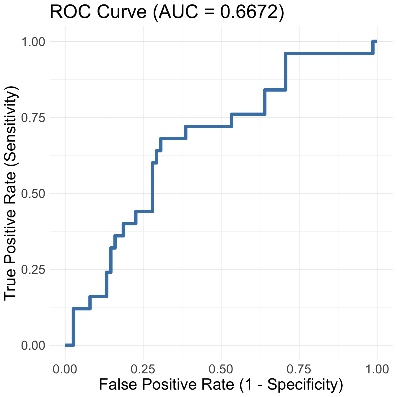
Code
ggroc(roc_glow, colour = 'steelblue', size = 2, legacy.axes = TRUE) +
  ggtitle(paste0('ROC Curve ', '(AUC = ', round(auc_glow, 4), ')')) +
  theme(text = element_text(size = 20)) +
  xlab("False Positive Rate (1 - Specificity)") +
  ylab("True Positive Rate (Sensitivity)")

Solutions / Resources (beyond our class right now)

Summary

  • Revisited model selection techniques and discussed how a binary outcome can be treated differently than a continuous outcome
  • Discussed association vs prediction modeling
  • Discussed classification: a type of machine learning!
  • Introduced penalized regression as a classification method
  • Performed penalized regression (specifically LASSO) to select a prediction model
  • Process presented today has major flaws
    • We did not tune our parameter
    • We did not perform cross validation

For your Lab 4

  • You can switch methods if you want!

  • You can use purposeful selection, like we did last quarter

    • If you want to focus on association modeling!

    • But you will need to include at least one interaction!!

    • A good way to practice this again if you struggled with it previously


  • You can try out LASSO regression

    • If you want to focus on prediction modeling!
    • And if you want to stretch your R coding skills