Lab 2: Feedback and Discussion

Nicky Wakim

2026-04-29

Notes from the TAs

• Please make sure to state which model building strategy you are using!
• TAs say your interpretations have been great!

Can I make this numeric?

• I’ve been getting this question for a few variables
• Some variables that might seem like we can convert to numeric
  • PPEDUCAT
  • PPINCIMP
  • NUM_CHILD_HH
  • NUM_OWN_CHILD
  • NUM_FAM_SIZE

 

• To convert a categorical variable to numeric, we need to convince ourselves that the categorical variable has a linear relationship with the log-odds of food insecurity

• How do we do that?

Check linearity!

• When we treat a predictor as continuous, we need to make sure we have linearity between the predictor and log-odds

• Easier to test this by fitting a logistic regression with the predictor

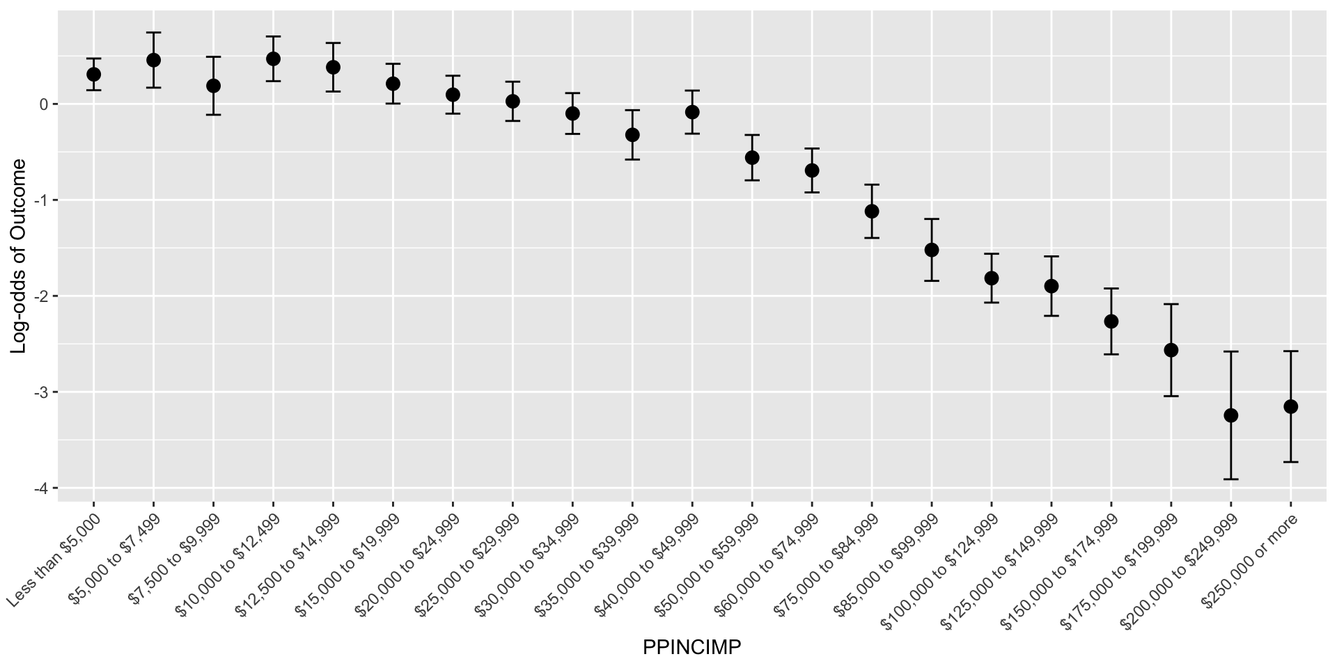
• Test linearity by fitting logistic regression with the predictor, then visually examining if predicted log-odds follows roughly linear pattern

 

• Let’s test this out with income

Set up the predicted log-odds

• First, I run a logistic regression model with PPINCIMP and FOOD_INSEC

income_glm = wbns3 %>% glm(formula = FOOD_INSEC ~ PPINCIMP, family = binomial)

• Then I use predict() to calculate the log-odds for each category

newdata = data.frame(PPINCIMP = levels(wbns3$PPINCIMP)) 
pred = predict(income_glm, newdata, se.fit=T, type = "link")

pred_link = data.frame(PPINCIMP = levels(wbns3$PPINCIMP), 
                       Pred = pred$fit, 
                       LL_CI1 = pred$fit - qnorm(1-0.05/2) * pred$se.fit, 
                       UL_CI1 = pred$fit + qnorm(1-0.05/2) * pred$se.fit) %>% 
  mutate(PPINCIMP = factor(PPINCIMP, levels = levels(wbns3$PPINCIMP)))

Now I can plot the log-odds vs. income: what do we notice??

ggplot() + 
  labs(y = "Log-odds of Outcome") +
  geom_point(data = pred_link, aes(x = PPINCIMP, y=Pred), size=3) +
  geom_errorbar(data = pred_link, aes(x = PPINCIMP, y=Pred, ymin = LL_CI1, ymax = UL_CI1), width = 0.25) +
  theme(axis.text.x = element_text(angle = 45, hjust = 1))

So I need to go back and map the levels to their midpoints

wbns4 <- wbns3 %>%
  mutate(income_midpoint = case_when(
    PPINCIMP == "Less than $5,000"     ~ 2500,
    PPINCIMP == "$5,000 to $7,499"     ~ 6250,
    PPINCIMP == "$7,500 to $9,999"     ~ 8750,
    PPINCIMP == "$10,000 to $12,499"   ~ 11250,
    PPINCIMP == "$12,500 to $14,999"   ~ 13750,
    PPINCIMP == "$15,000 to $19,999"   ~ 17500,
    PPINCIMP == "$20,000 to $24,999"   ~ 22500,
    PPINCIMP == "$25,000 to $29,999"   ~ 27500,
    PPINCIMP == "$30,000 to $34,999"   ~ 32500,
    PPINCIMP == "$35,000 to $39,999"   ~ 37500,
    PPINCIMP == "$40,000 to $49,999"   ~ 45000,
    PPINCIMP == "$50,000 to $59,999"   ~ 55000,
    PPINCIMP == "$60,000 to $74,999"   ~ 67500,
    PPINCIMP == "$75,000 to $84,999"   ~ 80000,
    PPINCIMP == "$85,000 to $99,999"   ~ 92500,
    PPINCIMP == "$100,000 to $124,999" ~ 112500,
    PPINCIMP == "$125,000 to $149,999" ~ 137500,
    PPINCIMP == "$150,000 to $174,999" ~ 162500,
    PPINCIMP == "$175,000 to $199,999" ~ 187500,
    PPINCIMP == "$200,000 to $249,999" ~ 225000,
    PPINCIMP == "$250,000 or more"     ~ 300000
  ))

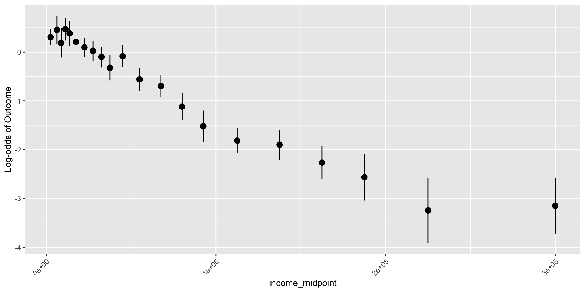
Do same prediction, but now inclue midpoints!

newdata = data.frame(PPINCIMP = levels(wbns4$PPINCIMP)) 
pred = predict(income_glm, newdata, se.fit=T, type = "link")

pred_link = data.frame(PPINCIMP = levels(wbns4$PPINCIMP), 
                       income_midpoint = sort(unique(wbns4$income_midpoint)), 
                       Pred = pred$fit, 
                       LL_CI1 = pred$fit - qnorm(1-0.05/2) * pred$se.fit, 
                       UL_CI1 = pred$fit + qnorm(1-0.05/2) * pred$se.fit) %>% 
  mutate(PPINCIMP = factor(PPINCIMP, levels = levels(wbns4$PPINCIMP)))

And plot again with midpoints!

ggplot() + 
  labs(y = "Log-odds of Outcome") +
  geom_point(data = pred_link, aes(x = income_midpoint, y=Pred), size=3) +
  geom_errorbar(data = pred_link, aes(x = income_midpoint, y=Pred, ymin = LL_CI1, ymax = UL_CI1), width = 0.25) +
  theme(axis.text.x = element_text(angle = 45, hjust = 1))

Now to peer discussion

Get into groups of 2-4ish

• Try to group with people with whos you do not already work on labs
• Introduce yourself if you do not know each other
• Share you html documents with each other (email, airdrop, etc.)

Introduce Research Question

• Share your research question with each other!
  • Should be using the same outcome + your main variable
• Share your other variables

 

Discuss your confounders/effect modifiers

• Does not need to have a causal framework
• Do you think we need to adjust for certain variables?
• Do you think there will be interactions?
• If you think there are interactions, try to narrow it down to 1-2 variables

Contingency tables + bivariate analysis

• Based on your reasoning in the previous activity and the tables/plots, do you think we need to adjust for any variables?
• What trends are you seeing?
• Do you have any cells with low counts?

Simple logistic regression

• Does everyone have the correct interpretations of the estimated odds ratios?
• What’s your reference group?
• What trends are you seeing?

Predicted Probabilities

• Let’s just check each other’s code and probabilities
• What would your predicted probabilities look like if you had a confounder? effect modifier?