Lesson 4: Measurements of Association and Agreement
2025-04-07
Relationship Between RR and OR (2/2)
An example where a disease rare over the whole sample (~1%), but …
- \(\widehat{OR}\) is not a good estimate of \(\widehat{RR}\) in “rare” disease
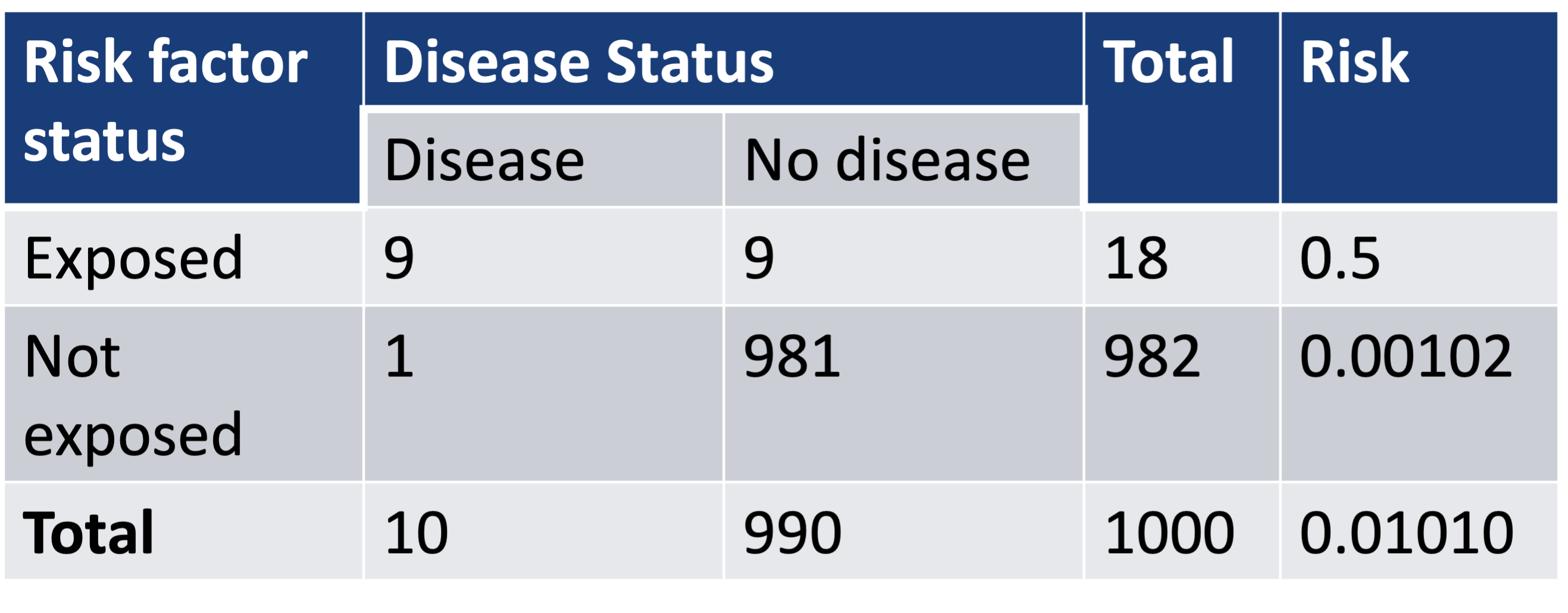
- \(\widehat{p}_1\) is 0.5: thus \(\widehat{OR}\) and \(\widehat{RR}\) are very different
\[\widehat{RR}=\frac{0.5}{0.00102}=490 \text{ and } \widehat{OR} = \frac{0.5(1-0.5)}{0.00102(1-0.00102)}=981\]
RR in retrospective case-control study (2/3)
- Assume a 1:2 case-control study summarized in below table:
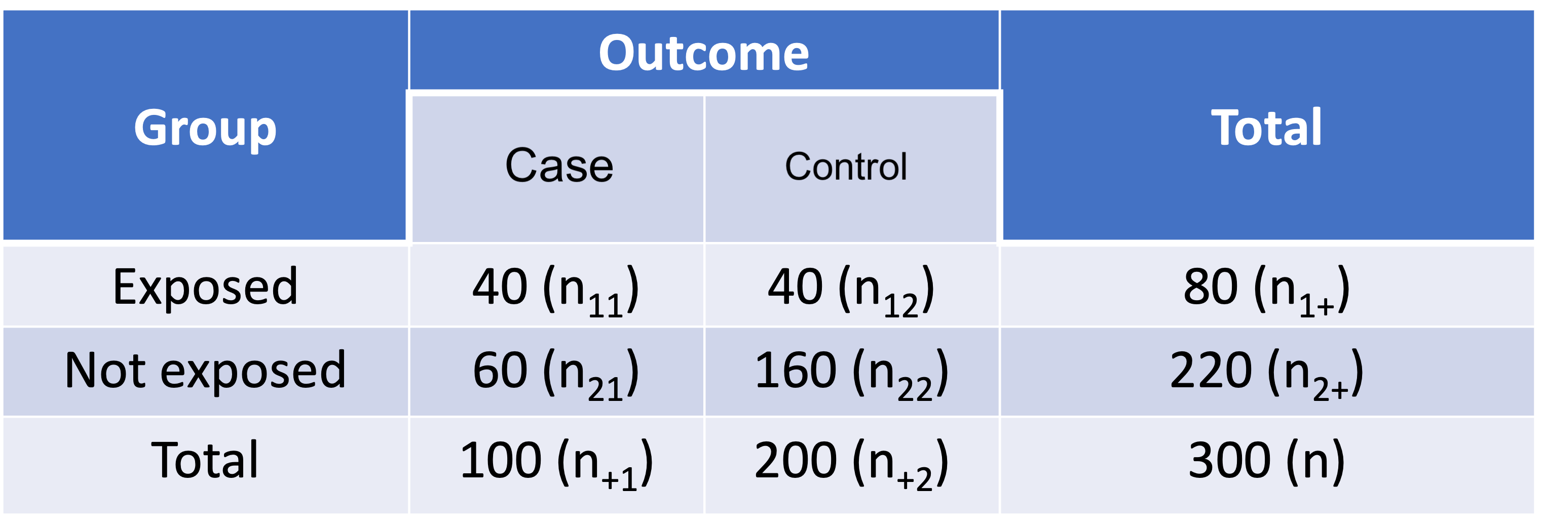
- Assume we compute the RR as if it is from a cohort study:
\[\widehat{RR}=\frac{\widehat{p_1}}{\widehat{p_2}}=\frac{n_{11}/n_{1+}}{n_{21}/n_{2+}}=\frac{40/80}{60/220}=1.8333\]
RR in prospective cohort study
- In real world, the proportion of controls (not diseased) is typically much higher. Assume the table below shows the proportion in the population in a cohort study
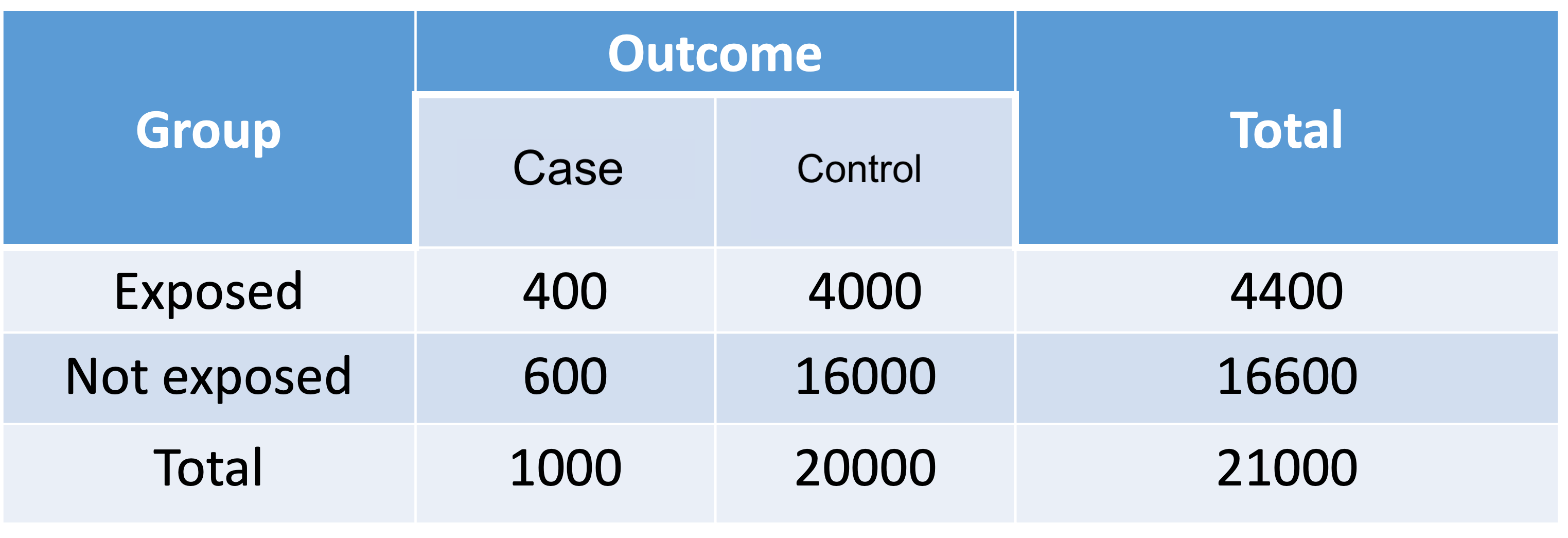
- The estimated RR for the patient population is:
\[\widehat{RR}=\frac{\widehat{p_1}}{\widehat{p_2}}=\frac{400/4400}{600/16600}=2.5152\]
OR in retrospective case-control study
While we cannot estimate RR from a case-control study, we can still estimate OR for case-control study
OR does not require us to distinguish between the outcome variable and explanatory variable in the contingency table
- AKA: Odds ratio of disease comparing exposed to not exposed is same as odds ratio of being exposed comparing diseased and not diseased
For case-control study where the probability of having outcome is small, the \(\widehat{OR}\) is a nice approximation to \(\widehat{RR}\)
For the 1:2 case-control table: \(\widehat{OR}=\frac{40\cdot160}{40\cdot60} = 2.667\)
Population cohort study: \(\widehat{RR}=2.5152\)
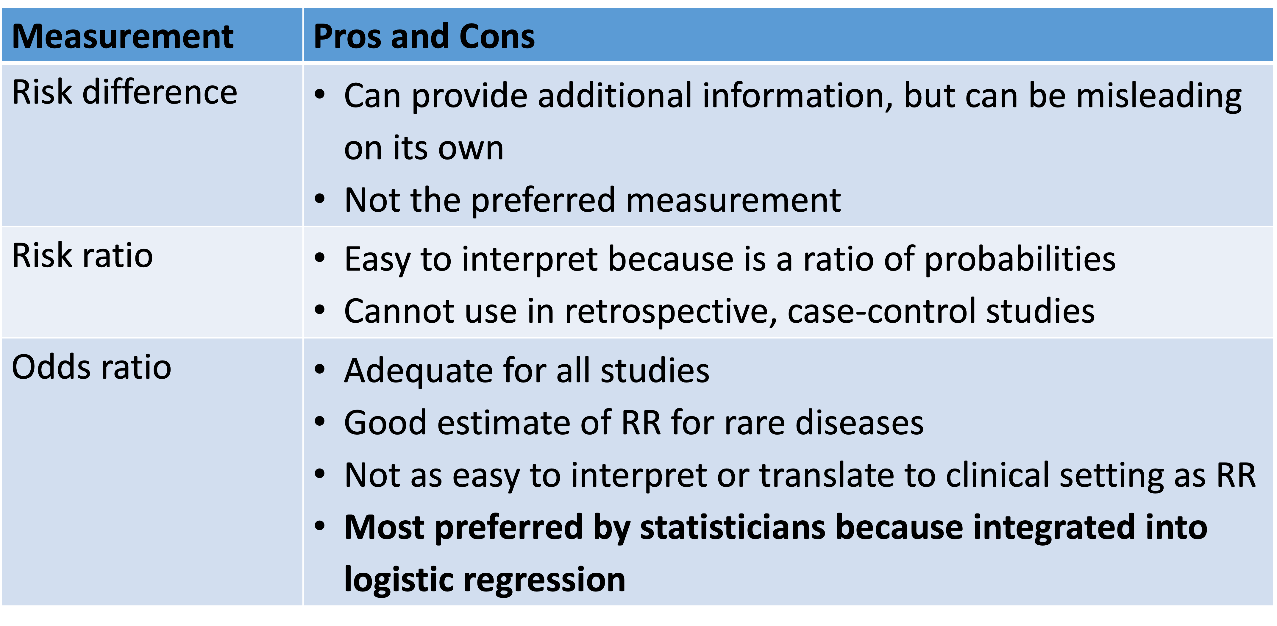
Which measurement should one use?
Let’s get our mood data down!
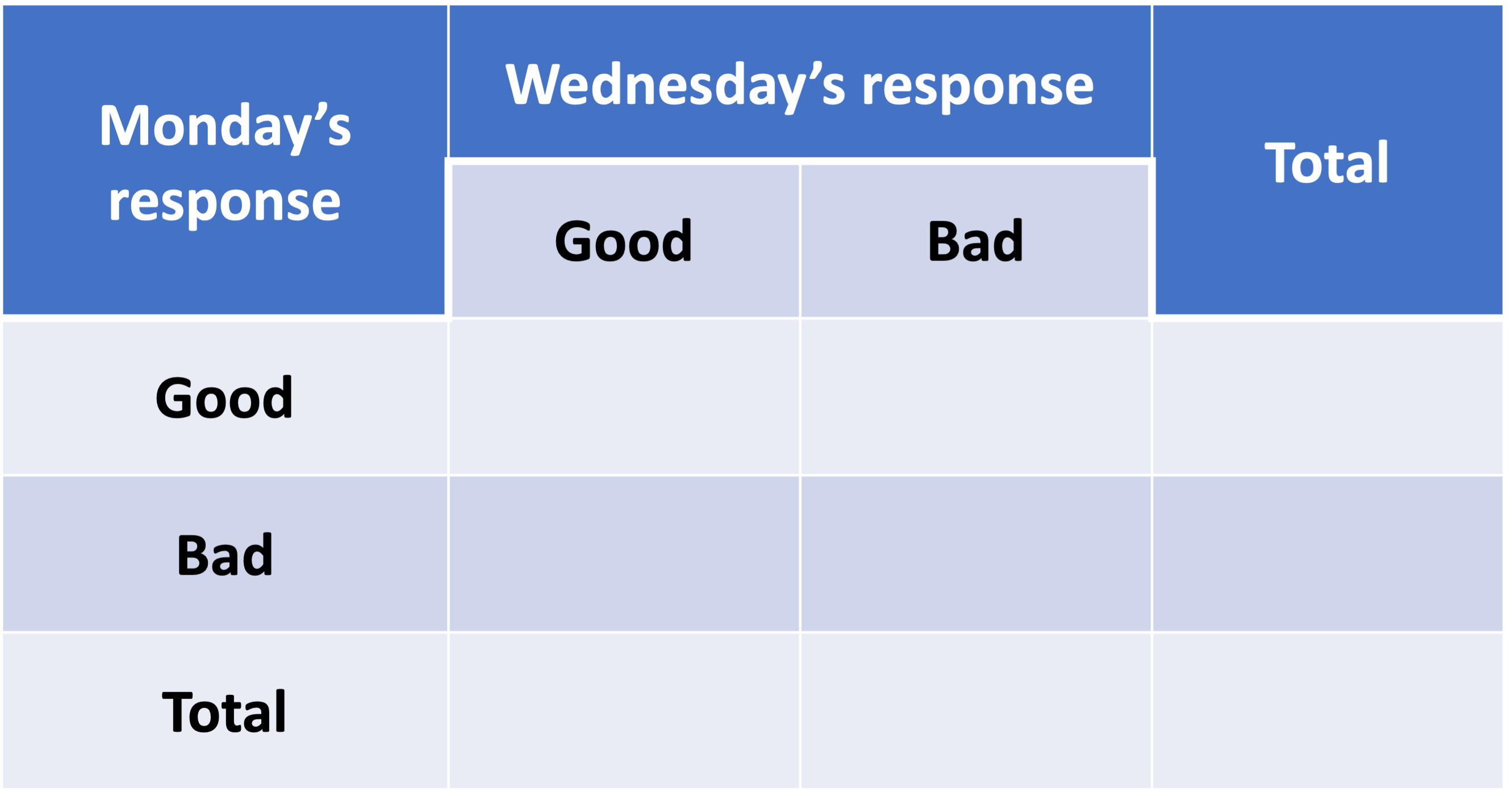
Example: Our moods (1/3)
Agreement of surveys
Compute the point estimate and 95% confidence interval for the agreement between our Monday and Wednesday moods.
Needed steps:
- Compute the kappa statistic
- Find confidence interval of kappa
- Interpret the estimate
Example: Our moods (2/3)
Agreement of surveys
Compute the point estimate and 95% confidence interval for the agreement between our Monday and Wednesday moods.
Needed steps:
1/2. Compute the kappa statistic and find confidence interval of kappa
Example: Our moods (3/3)
Agreement of surveys
Compute the point estimate and 95% confidence interval for the agreement between our Monday and Wednesday moods.
Needed steps:
- Interpret the estimate
The kappa statistic is ____________ (95% CI: _____________, _____________), indicating ______________ agreement.
Since the 95% confidence interval does/does not contain 0, we have/do not have sufficient evidence that there is _________ agreement between our mood on Monday and our mood on Wednesday.
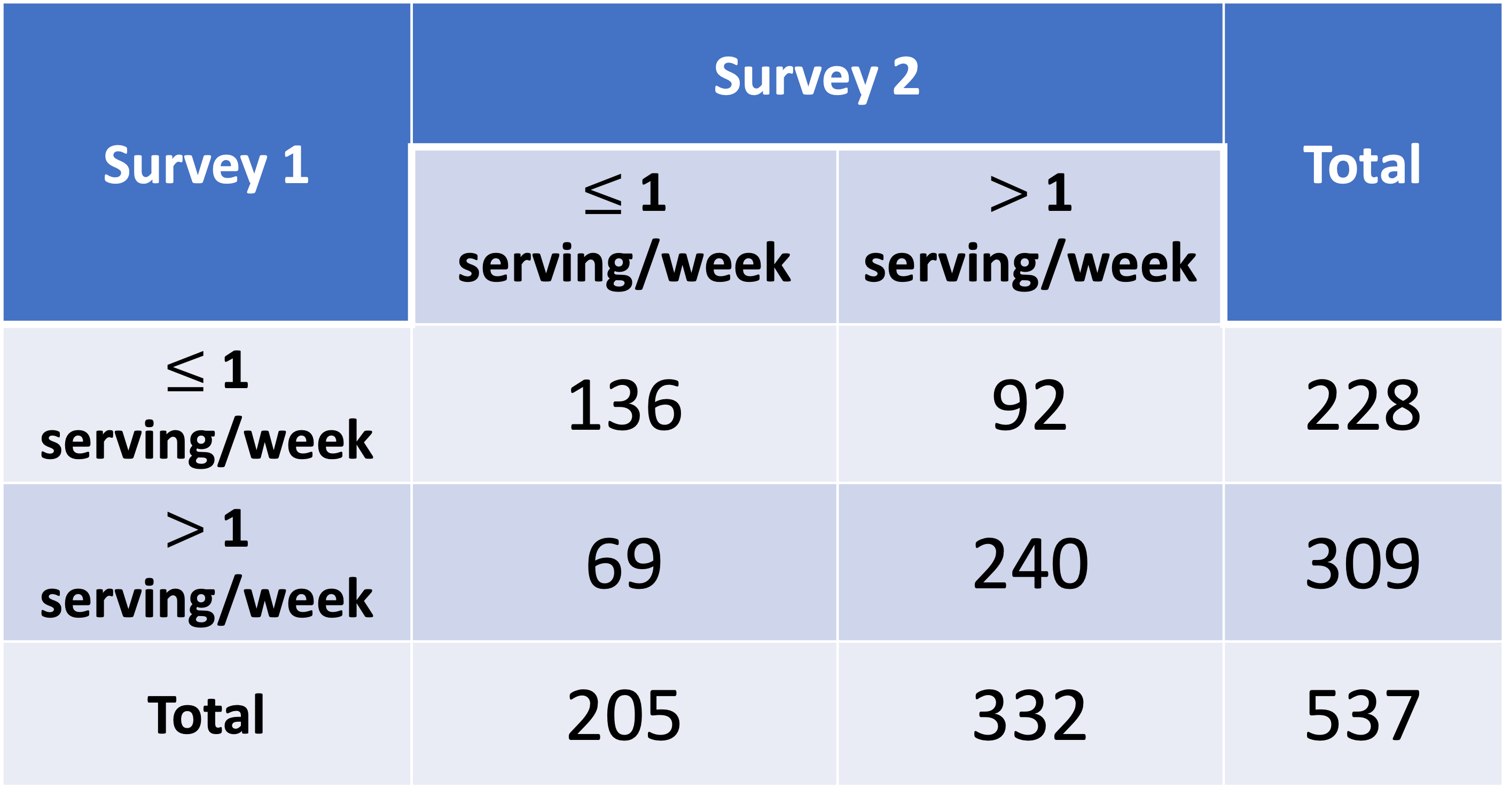
Just in case our data doesn’t work out: Beef Consumption in Survey
A diet questionnaire was mailed to 537 female American nurses on two separate occasions several months apart. The questions asked included the quantities eaten of more than 100 separate food items. The data from the two surveys for the amount of beef consumption are presented in the below table. How can reproducibility of response for the beef-consumption data be quantified?
Example: Beef Consumption in Survey (1/3)
Agreement of surveys
Compute the point estimate and 95% confidence interval for the agreement between beef consumption surveys. Similar to question: Are results reproducible for the beef-consumption in the survey?
Needed steps:
- Compute the kappa statistic
- Find confidence interval of kappa
- Interpret the estimate
Example: Beef Consumption in Survey (2/3)
Agreement of surveys
Compute the point estimate and 95% confidence interval for the agreement between beef consumption surveys. Similar to question: Are results reproducible for the beef-consumption in the survey?
Needed steps:
1/2. Compute the kappa statistic and find confidence interval of kappa
Example: Beef Consumption in Survey (3/3)
Agreement of surveys
Compute the point estimate and 95% confidence interval for the agreement between beef consumption surveys. Similar to question: Are results reproducible for the beef-consumption in the survey?
Needed steps:
- Interpret the estimate
The kappa statistic is 0.378 (95% CI: 0.298, 0.459), indicating fair agreement.
Since the 95% confidence interval does not contain 0, we have sufficient evidence that there is fair agreement between the surveys for beef consumption. The survey is not reliably reproducible since we did not achieve excellent agreement.