Lesson 14: Model Building
With an emphasis on prediction
2025-05-14
Bias-variance trade off
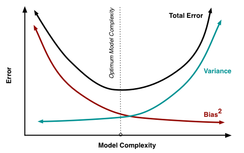
Recall from 512/612: MSE can be written as a function of the bias and variance
\[ MSE = \text{bias}\big(\widehat\beta\big)^2 + \text{variance}\big(\widehat\beta\big) \]
- We no longer use MSE in logistic regression to find the best fit model, BUT the idea between the bias and variance trade off holds!
For the same data:
More covariates in model: less bias, more variance
- Potential overfitting: with new data does our model still hold?
Less covariates in model: more bias, less variance
- More bias bc more likely that were are not capturing the true underlying relationship with less variables
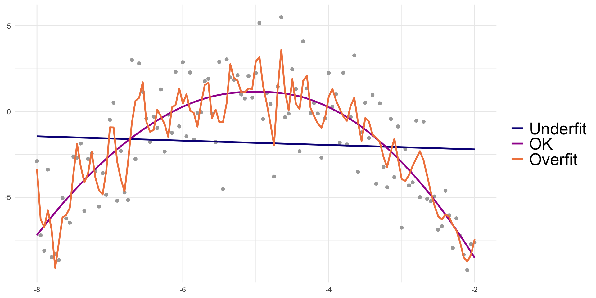
Visual of overfitting and underfitting data
From Data Science in a Box:
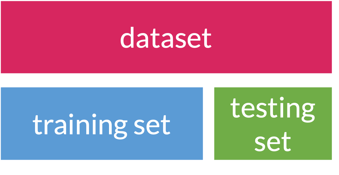
Step 1: Splitting data
Training: act of creating our prediction model based on our observed data
- Supervised: Means we keep information on our outcome while training
- Testing: act of measuring the predictive accuracy of our model by trying it out on new data
When we use data to create a prediction model, we want to test our prediction model on new data
- Helps make sure prediction model can be applied to other data outside of the data that was used to create it!
- So an important first step in prediction modeling is to split our data into a training set and a testing set!
Step 1: Splitting data
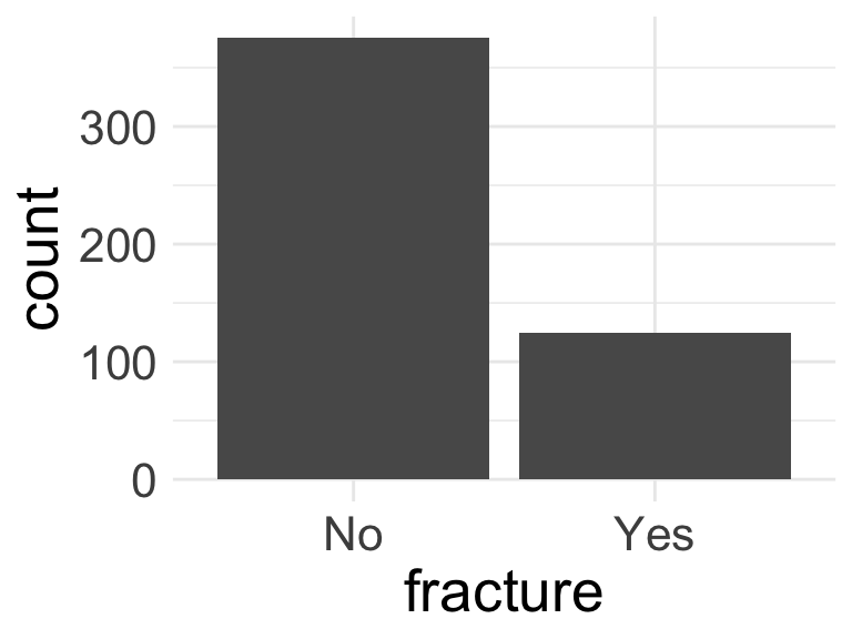
When splitting data, we need to be conscious of the proportions of our outcomes
Is there imbalance within our outcome?
We want to randomly select observations but make sure the proportions of No and Yes stay the same
We stratify by the outcome, meaning we pick Yes’s and No’s separately for the training set
Side note: took out
bmiandweightbc we have multicollinearity issues- Combo of I hate these variables and my previous work in the LASSO identified these as not important
Step 2: Fit LASSO: Main effects: Identify variables
library(vip)
vi_data_main = glow_fit_main %>%
    pull_workflow_fit() %>%
    vi(lambda = 0.002) %>% # vi: variable importance
    filter(Importance != 0)
vi_data_main
# A tibble: 9 × 3
Variable Importance Sign
<chr> <dbl> <chr>
1 raterisk_Greater 0.535 POS
2 momfrac_Yes 0.526 POS
3 priorfrac_Yes 0.485 POS
4 raterisk_Same 0.413 POS
5 smoke_Yes 0.344 NEG
6 premeno_Yes 0.267 POS
7 fracscore 0.196 POS
8 armassist_Yes 0.138 POS
9 height 0.0370 NEG 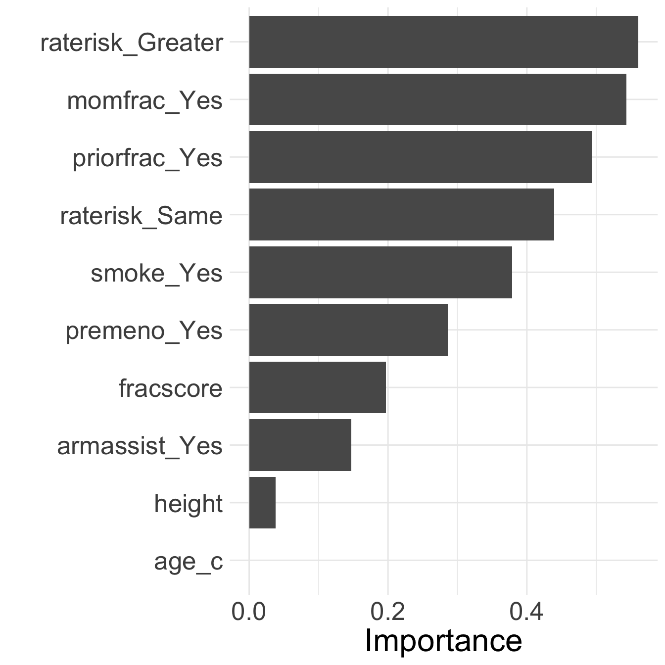
- Looks like age is removed!
Step 3: Prediction on testing set
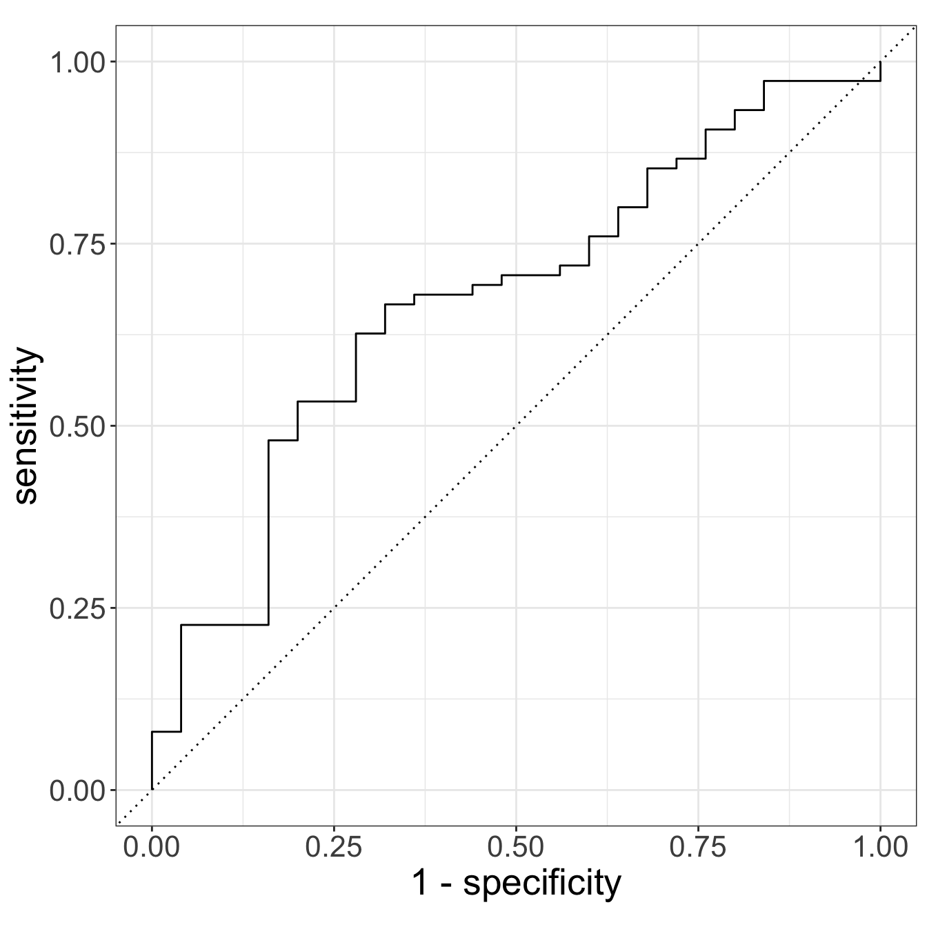
Step 3: Prediction on testing set
# A tibble: 1 × 3
  .metric .estimator .estimate
  <chr>   <chr>          <dbl>
1 roc_auc binary         0.672
Why is this AUC worse than the one we saw with prior fracture, age, and their interaction?
- Only 1 training and testing set: can overfit training and perform poorly on testing
- We did not tune our penalty
- Our testing set only has 100 observations!

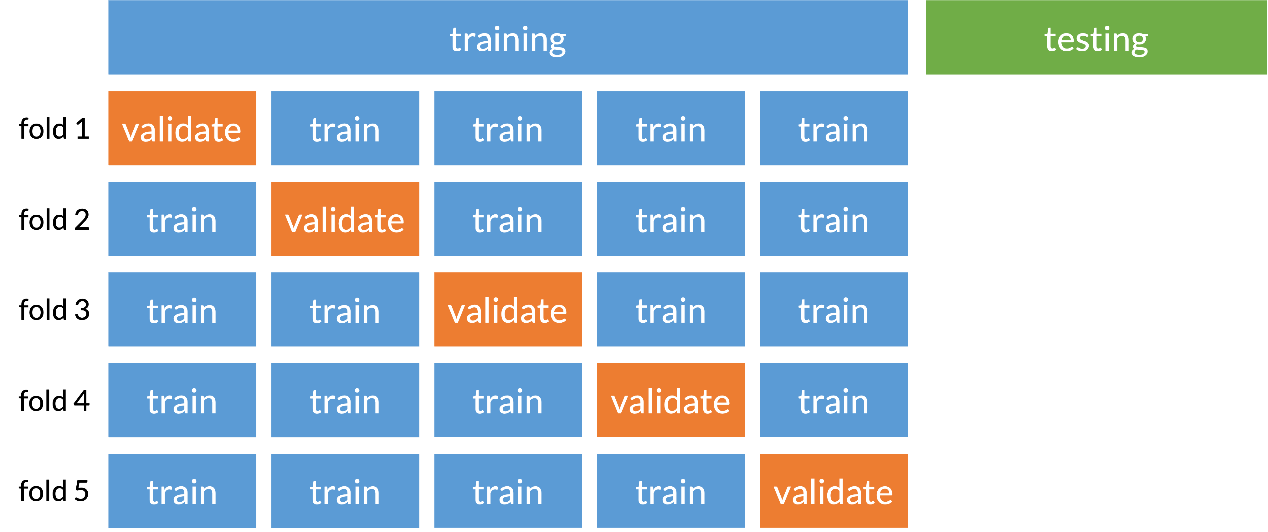
Cross-validation (specifically k-fold)
Prevents overfitting to one set of training data
Split data into folds that train and validate model selection
Basically subsection of training and testing (called validating) before truly testing on our original testing set