Lesson 15: Other types of categorical regression

Nicky Wakim

2025-05-21

Learning Objectives

  1. Review Generalized Linear Models and how we can branch to other types of regression.

  2. Identify outcome, examples, population model, and interpretations for different generalized linear models.

Learning Objectives

  1. Review Generalized Linear Models and how we can branch to other types of regression.
  1. Identify outcome, examples, population model, and interpretations for different generalized linear models.

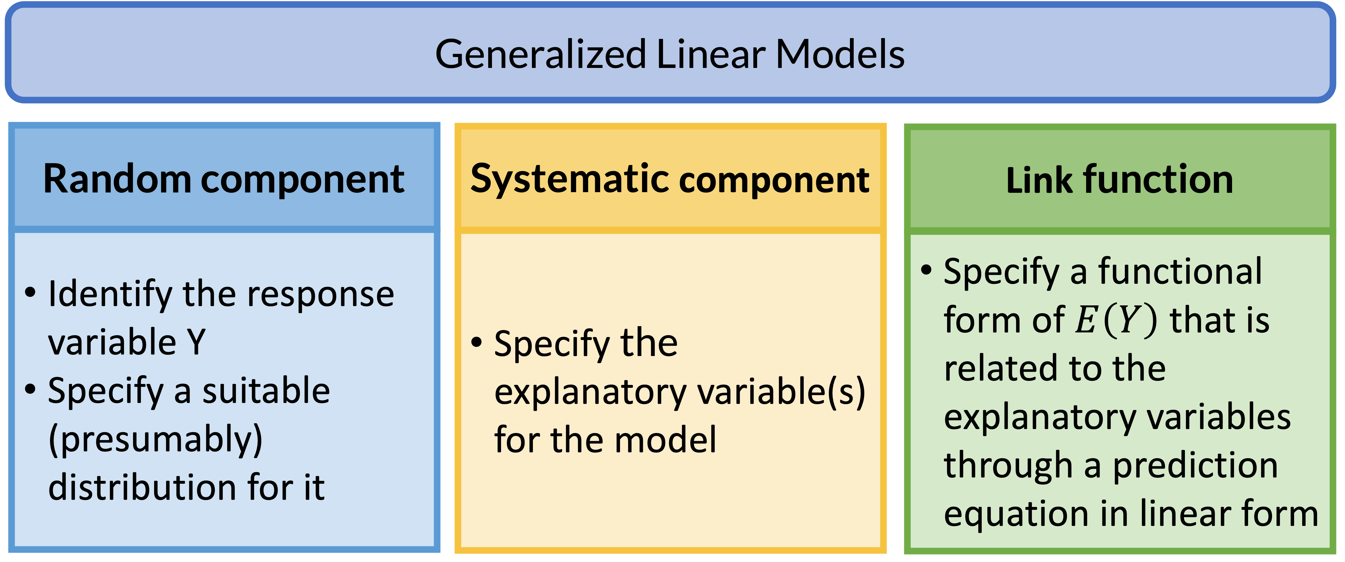
Review: Generalized Linear Models (GLMs)

GLM: Random Component

  • The random component specifies the response variable \(Y\) and selects a probability distribution for it


  • Basically, we are just identifying the distribution for our outcome

    • If Y is binary: assumes a binomial distribution of Y

    • If Y is count: assumes Poisson or negative binomial distribution of Y

    • If Y is continuous: assumea Normal distribution of Y

GLM: Systematic Component

  • The systematic component specifies the explanatory variables, which enter linearly as predictors \[\beta_0+\beta_1X_1+\ldots+\beta_kX_k\]


  • Above equation includes:

    • Centered variables
    • Interactions
    • Transformations of variables (like squares)


  • Systematic component is the same as what we learned in Linear Models

Poll Everywhere Question 1

Learning Objectives

  1. Review Generalized Linear Models and how we can branch to other types of regression.
  1. Identify outcome, examples, population model, and interpretations for different generalized linear models.

Linear regression

  • Outcome type: continuous


  • Example outcomes:
    • Height
    • IAT score
    • Heart rate
  • Population model

\[ E(Y \mid X) = \mu = \beta_0 + \beta_1 X\]

  • Interpretations
    • The change in average \(Y\) for every 1 unit increase in \(X\)

Linear regression: Process for data analysis

Model Selection

  • Building a model

  • Selecting variables

  • Prediction vs interpretation

  • Comparing potential models

Model Fitting

  • Find best fit line

  • Using OLS in this class

  • Parameter estimation

  • Categorical covariates

  • Interactions

Model Evaluation

  • Evaluation of model fit
  • Testing model assumptions
  • Residuals
  • Transformations
  • Influential points
  • Multicollinearity

Model Use (Inference)

  • Inference for coefficients
  • Hypothesis testing for coefficients
  • Inference for expected \(Y\) given \(X\)
  • Prediction of new \(Y\) given \(X\)

Logistic regression

  • Outcome type: binary, yes or no


  • Example outcomes:
    • Food insecurity
    • Disease diagnosis for patient
    • Fracture
  • Population model

\[ \text{logit}(\mu) = \text{logit}(\pi(X)) = \beta_0 + \beta_1 X\]

  • Interpretations
    • The log-odds ratio for every 1 unit increase in \(X\)
    • \(\text{exp}\big(\beta_1\big)\) is odds ratio for every 1 unit increase in \(X\)

Logistic regression: Process for data analysis

Model Selection

  • Build a model

  • Select variables

  • Prediction vs association

  • Comparing potential models

Model Fitting

  • Find model that maximizes likelihood function

  • Parameter estimation (MLEs)

  • Categorical covariates

  • Interactions

Model Evaluation

  • Evaluation of model fit
  • Check model assumptions
  • Transformations
  • Influential points
  • Multicollinearity
  • Overdispersion

Model Use (Inference)

  • Inference for odds ratios
  • Hypothesis testing for odds ratios
  • Inference for expected \(\pi\) given \(X\)
  • Prediction of new \(Y\) given \(X\)

Log-binomial Regression

  • Outcome type: binary, yes or no


  • Example outcomes:
    • Food insecurity
    • Disease diagnosis for patient
    • Fracture
  • Population model

\[ \log(\mu) = \text{log}(\pi(X)) = \beta_0 + \beta_1 X\]

  • Interpretations
    • We have log of probability on the left
    • So exponential of our coefficients will be risk ratio

Poisson Regression

  • Outcome type: Counts or rates


  • Example outcomes:
    • Number of children in household
    • Number of hospital admissions
    • Rate of incidence for COVID in US counties
  • Population model

\[ \log(\mu) = \log(\lambda) = \beta_0 + \beta_1 X\]

  • Interpretations
    • The count (or rate) ratio for every 1 unit increase in \(X\)

Multinomial logistic regression

  • Outcome type: multi-level categorical, no inherent order


  • Example outcomes:
    • Blood type
    • US region (from WBNS)
    • Primary site of lung cancer (upper lobe, lower lobe, overlapped, etc.)
  • We have additional restriction that the multiple group probabilities sum to 1
  • Population models\[ \log \left(\dfrac{\mu_{\text{group } 2}}{\mu_{\text{group } 1}} \right) = \beta_0 + \beta_1 X\] \[ \log \left(\dfrac{\mu_{\text{group } 3}}{\mu_{\text{group } 1}} \right) = \beta_0 + \beta_1 X\]

  • Interpretations

    • Basically fitting two binary logistic regressions at same time!
    • First equation: how a one unit change in \(X\) changes the log-odds of going from group 1 to group 2
    • Second equation: how a one unit change in \(X\) changes the log-odds of going from group 1 to group 3

Ordinal logistic regression

  • Outcome type: multi-level categorical, with inherent order
  • Example outcomes:
    • Satisfaction level (likert scale)
    • Pain level
    • Stages of cancer


  • When these variables are predictors, we are pretty lenient about treating them as continuous
    • We must be VERY STRICT when they are outcomes
    • They do not meet the assumptions we place on continuous outcomes in linear regression!!
  • We have additional restriction that the multiple group probabilities sum to 1
  • Population models , with levels \(k = 1, 2, 3, ..., K\)

\[ \log \left(\dfrac{P(Y \leq 1)}{P(Y > 1)} \right) = \beta_0 + \beta_1 X\] \[ \log \left(\dfrac{P(Y \leq k)}{P(Y > k)} \right) = \beta_0 + \beta_1 X\]

  • Interpretations
    • Basically fitting \(K\) binary logistic regressions at same time!
    • First equation: how a one unit change in \(X\) changes the log-odds of going from group 1 to any other group
    • Second equation: how a one unit change in \(X\) changes the log-odds of going from group 1 or 2 to group 3 or above

Resources

Poisson Regression resources

Multinomial logistic regression resources

Even more regressions…

Dist’n of Y Typical uses Link name Link function Common name
Bernoulli / Binomial outcome of single yes/no occurrence Probit \(g(\mu)=\Phi^{-1}(\mu)\) Probit regression
Bernoulli / Binomial outcome of single yes/no occurrence Complementary log-log \(g(\mu)=\log(-\log(1-\mu))\) Complementary log-log regression
Multinomial outcome of single occurence with K > 2 options, nominal Probit \(g(\mu)=\Phi^{-1}(\mu)\) Multinomial probit regression
Multinomial outcome of single occurence with K > 2 options, ordinal Probit \(g(\mu)=\Phi^{-1}(\mu)\) Ordered probit regression

More regression resources

General resources