Lesson 16: Log-binomial Regression

Nicky Wakim

2025-05-28

Learning Objectives

  1. Revisit the key distinctions between logistic and log-binomial regression.
  2. Interpret and visualize coefficient estimates, risk ratios, and predicted probabilities.

Learning Objectives

  1. Revisit the key distinctions between logistic and log-binomial regression.
  1. Interpret and visualize coefficient estimates, risk ratios, and predicted probabilities.

Log-binomial Regression

  • Outcome type: binary, yes or no


  • Example outcomes:
    • Food insecurity
    • Disease diagnosis for patient
    • Fracture
  • Population model

\[ \log(\mu) = \beta_0 + \beta_1 X\]

  • Interpretations
    • We have log of probability on the left
    • So exponential of our coefficients will be risk ratio

Logistic regression vs. log-binomial regression

  • Outcome is the same: still a binary variable
    • Still modeling with probability of event: \(P(Y=1|X)\)
  • Logistic = logit = log of odds
    • Aim to get odds ratios for interpretation (exponential of coefficients)
    • You can convert the odds ratios to risk ratios
  • Log-binomial = log of probability
    • Aim to get risk ratio or prevalence ratio (exponential of coefficients)


  • Disadvantage of log-binomial
    • Left hand side (aka \(\log(\pi(X))\)) is only a positive value, while right hand side can range from \(-\infty\) to \(\infty\)
    • Prone to issues while trying to fit the model!

A few classes ago: GLOW Study with interactions

  • Outcome variable: any fracture in the first year of follow up (FRACTURE: 0 or 1)

  • Risk factor/variable of interest: history of prior fracture (PRIORFRAC: 0 or 1)

  • Potential confounder or effect modifier: age (AGE, a continuous variable)


  • Fit a logistic regression model with interactions:
\[\begin{aligned} \text{logit}\left(\pi(\mathbf{X})\right) & = \beta_0 + \beta_1 \cdot I(\text{PF}= \text{``Yes"}) + \beta_2 \cdot Age + \beta_3 \cdot I(\text{PF} = \text{``Yes"}) \cdot Age \\ \text{logit}\left(\widehat\pi(\mathbf{X})\right) & = \widehat\beta_0 + \widehat\beta_1 \cdot I(\text{PF}= \text{``Yes"}) + \widehat\beta_2 \cdot Age + \widehat\beta_3 \cdot I(\text{PF} = \text{``Yes"}) \cdot Age \\ \text{logit}\left(\widehat\pi(\mathbf{X})\right) & = -1.376 + 1.002 \cdot I(\text{PF}=\text{``Yes"}) + 0.063 \cdot Age - 0.057 \cdot I(\text{PF}=\text{``Yes"}) \cdot Age \end{aligned}\]

Logistic regression: Reporting results of GLOW Study with interactions

  • Remember our main covariate is prior fracture, so we want to focuse on how age changes the relationship between prior fracture and a new fracture!

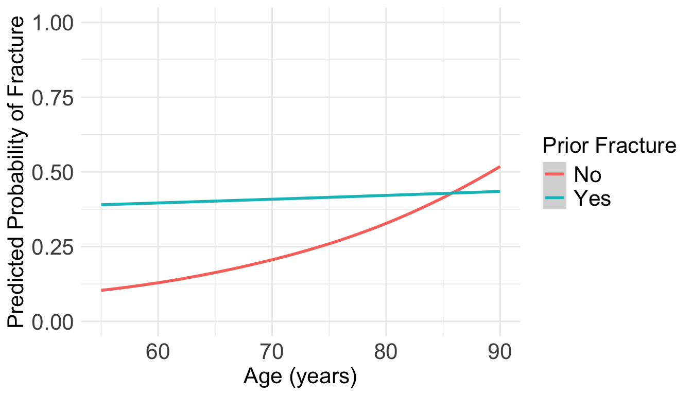
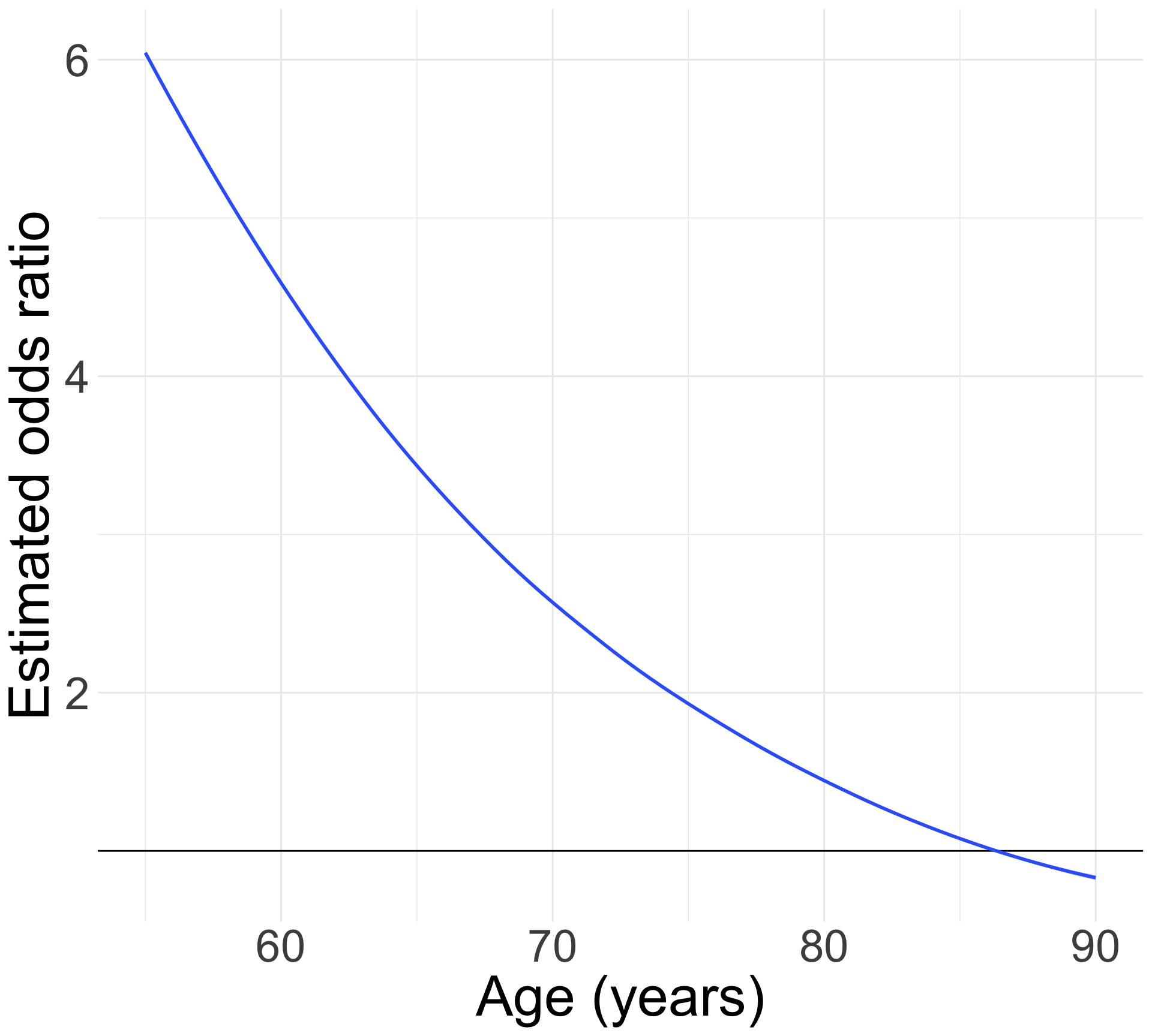
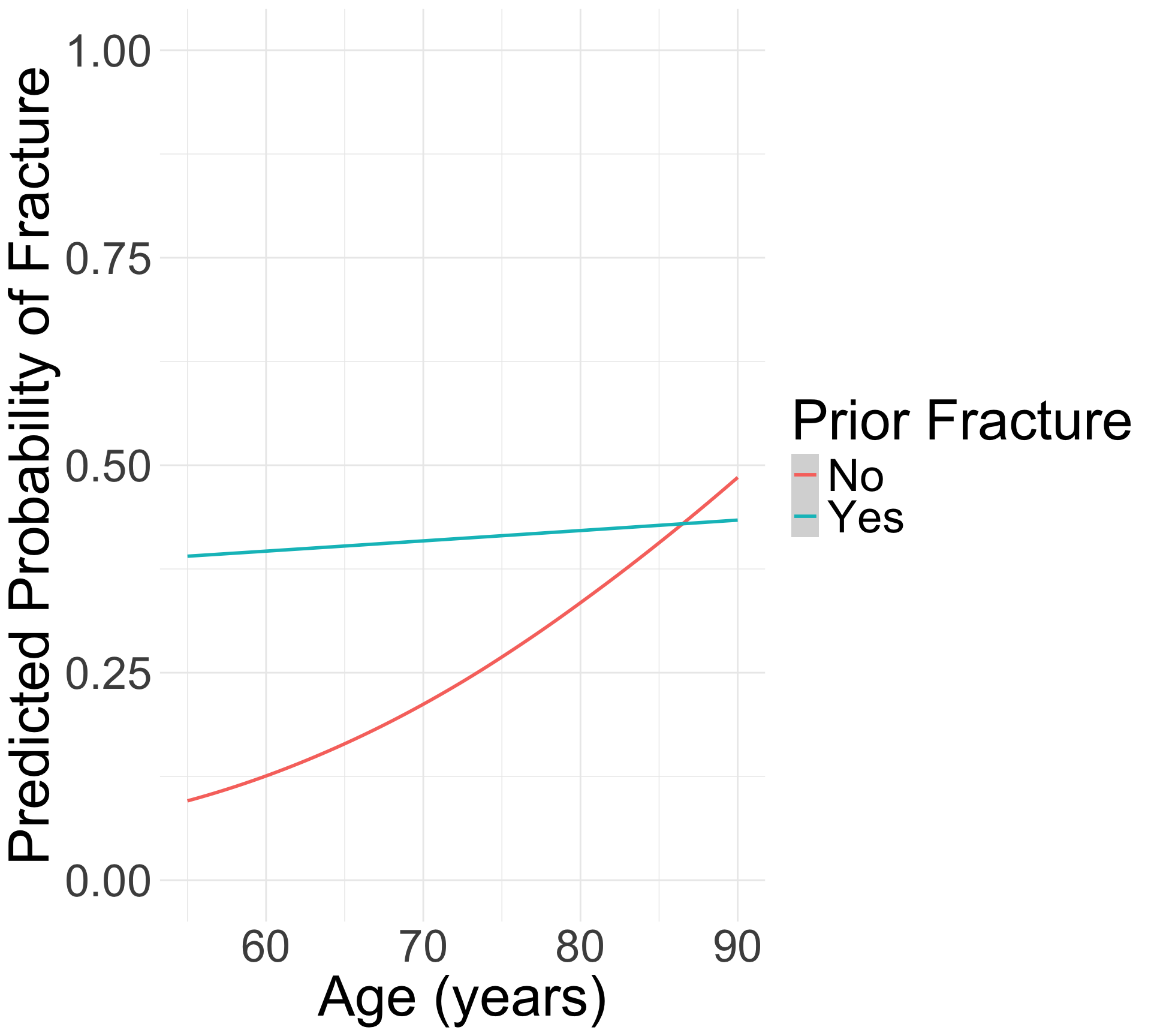
For individuals 69 years old, the estimated odds of a new fracture for individuals with prior fracture is 2.72 times the estimated odds of a new fracture for individuals with no prior fracture (95% CI: 1.70, 4.35). As seen in Figure 1 (a), the odds ratio of a new fracture when comparing prior fracture status decreases with age, indicating that the effect of prior fractures on new fractures decreases as individuals get older. In Figure 1 (b), it is evident that for both prior fracture statuses, the predict probability of a new fracture increases as age increases. However, the predicted probability of new fracture for those without a prior fracture increases at a higher rate than that of individuals with a prior fracture. Thus, the predicted probabilities of a new fracture converge at age [insert age here].

(a) Odds ratio of fracture outcome comparing prior fracture to no prior fracture
(b) Predicted probability of fracture
Figure 1: Plots of odds ratio and predicted probability from fitted interaction model

What would a log-binomial equivalent look like?

  • For the same GLOW data, we could fit a log-binomial model:

\[\text{log}\left(\widehat\pi(\mathbf{X})\right) = \widehat\beta_0 + \widehat\beta_1 \cdot I(\text{PF}= \text{``Yes"}) + \widehat\beta_2 \cdot Age + \widehat\beta_3 \cdot I(\text{PF} = \text{``Yes"}) \cdot Age \]

  • What does this look like in the glm function?
glow_log_binom = glow %>% glm(formula = fracture ~ priorfrac + age_c + priorfrac*age_c, 
                              family = binomial(link = "log"))
Table for coefficient estimates
tidy(glow_log_binom, conf.int = T) %>% 
  gt() %>% 
  tab_options(table.font.size = 30) %>%
  fmt_number(decimals = 3)
term estimate std.error statistic p.value conf.low conf.high
(Intercept) −1.625 0.106 −15.269 0.000 −1.846 −1.427
priorfracYes 0.727 0.159 4.570 0.000 0.404 1.034
age_c 0.046 0.011 4.217 0.000 0.025 0.066
priorfracYes:age_c −0.043 0.016 −2.710 0.007 −0.074 −0.012

Let’s start with a model with main effects only

  • Just so we have a simpler model as we first demostrate the log-binomial:

\[\text{log}\left(\widehat\pi(\mathbf{X})\right) = \widehat\beta_0 + \widehat\beta_1 \cdot I(\text{PF}= \text{``Yes"}) + \widehat\beta_2 \cdot Age \]

  • Run a logistic regression model using glm(): works!
glow2_logistic = glow %>% 
  glm(formula = fracture ~ priorfrac + age_c, 
                              family = binomial)


  • Run a log-binomial model using glm(): does not work!
glow2_log_binom = glow %>% 
  glm(formula = fracture ~ priorfrac + age_c, 
                              family = binomial(link = "log"))

Error: no valid set of coefficients has been found: please supply starting values

How to fix this?

  • We can fit the log-binomial model using logbin()
    • This function uses something called the EM algorithm to fit the data
    • Recall that glm uses an iteratively reweighted least squares algorithm
glow2_log_binom = logbin(formula = fracture ~ priorfrac + age_c, 
         data = glow)
  • Using logbin instead of glm will often fix the issue with fitting
    • But it does not work 100% of the time!
Table for coefficient estimates from logbin()
tidy(glow2_log_binom, conf.int = T) %>% 
  gt() %>% 
  tab_options(table.font.size = 33) %>%
  fmt_number(decimals = 3)
term estimate std.error statistic p.value conf.low conf.high
(Intercept) −1.595 0.103 −15.428 0.000 −1.798 −1.393
priorfracYes 0.545 0.159 3.416 0.001 0.232 0.857
age_c 0.026 0.008 3.104 0.002 0.009 0.042

Model tests: same as logistic regression

  • We would go through the same procedure as logistic regression
    • Because both models are rooted in the likelihood function!


  • Use LRT to test multiple variables OR one categorical variable with multiple levels


  • Use Wald test to construct confidence intervals
    • Or test one continuous or one binary variable

Learning Objectives

  1. Revisit the key distinctions between logistic and log-binomial regression.
  1. Interpret and visualize coefficient estimates, risk ratios, and predicted probabilities.

Interpreting risk ratios from log-binomial regression

  • Let’s say we ran the following model:

\[\text{log}\left(\widehat\pi(\mathbf{X})\right) = \widehat\beta_0 + \widehat\beta_1 \cdot I(\text{PF}= \text{``Yes"}) + \widehat\beta_2 \cdot Age\]

  • \(\exp(\beta_0)\): The risk of fracture (outcome event) for someone who had no prior fracture and is the mean age of 69 years old

  • \(\exp(\beta_1)\): The risk of fracture for someone who had a prior fracture is \(\exp(\beta_1)\) times the risk of fracture for someone who did not have a prior fracture, adjusting for age.

  • \(\exp(\beta_2)\): For every one year increase in age, the risk of fracture is \(\exp(\beta_2)\) times, adjusting for prior fracture.


*Recall that once I estimate the coefficients, my interpretations need to reflect that they are estimated by saying “estimated risk”

Interpretation of risk ratio: no interactions (1/2)

  • If we have no interactions in the model (using logbin):
glow_main = logbin(formula = fracture ~ priorfrac + age_c, data = glow)
  • Look at the exponential of the coefficients (risk ratio):
tidy(glow_main, conf.int = T, exponentiate = T) %>% 
  gt() %>% 
  tab_options(table.font.size = 35) %>%
  fmt_number(decimals = 3)
term estimate std.error statistic p.value conf.low conf.high
(Intercept) 0.203 0.103 −15.428 0.000 0.166 0.248
priorfracYes 1.724 0.159 3.416 0.001 1.261 2.356
age_c 1.026 0.008 3.104 0.002 1.010 1.043

Interpretation of risk ratio: no interactions (2/2)

term estimate std.error statistic p.value conf.low conf.high
(Intercept) 0.203 0.103 −15.428 0.000 0.166 0.248
priorfracYes 1.724 0.159 3.416 0.001 1.261 2.356
age_c 1.026 0.008 3.104 0.002 1.010 1.043
  • \(\exp(\widehat{\beta}_0)\): The estimated risk of fracture is 0.2 for someone who had no prior fracture and is the mean age of 69 years old

  • \(\exp(\widehat{\beta}_1)\): The estimated risk of fracture for someone who had a prior fracture is 1.72 times the estimated risk of fracture for someone who did not have a prior fracture, adjusting for age.

  • \(\exp(\widehat{\beta}_2)\): For every one year increase in age, the estimated risk of fracture is 1.03 times, adjusting for prior fracture.

    • OR: For every one year increase in age, the estimated risk of fracture increases 2.61%, adjusting for prior fracture.

Visualization: We can look at the log-risk

  • This will help us understand the model that we fit
  • Ultimately, we do not need a visualization of the risk ratio because the main effects model is constant across age
Table of coefficient estimates
tidy(glow_main) %>% 
  gt() %>% 
  tab_options(table.font.size = 30) %>%
  fmt_number(decimals = 3)
term estimate std.error statistic p.value
(Intercept) −1.595 0.103 −15.428 0.000
priorfracYes 0.545 0.159 3.416 0.001
age_c 0.026 0.008 3.104 0.002
Code to make the following plot
prior_age = expand_grid(priorfrac = c("No", "Yes"), age_c = (55:90)-69)
frac_pred_lb = predict(glow_main, prior_age, se.fit = F, type="link")
pred_glow_lb = prior_age %>% mutate(frac_pred = frac_pred_lb, 
                                  age = age_c + mean_age)

ggplot(pred_glow_lb) +
  geom_vline(xintercept = 69) +
  geom_smooth(method = "loess", aes(x = age, y = frac_pred, color = priorfrac)) +
  theme(text = element_text(size=35), title = element_text(size=22)) +
  labs(x = "Age (years)", y = "Estimated log-risk")

Interactions: interpretations and visualizations

\[\text{log}\left(\widehat\pi(\mathbf{X})\right) = \widehat\beta_0 + \widehat\beta_1 \cdot I(\text{PF}= \text{``Yes"}) + \widehat\beta_2 \cdot Age + \widehat\beta_3 \cdot I(\text{PF}= \text{``Yes"}) \cdot Age\]

glow3 = glow %>%
  mutate(interaction_PF_age = as.numeric(priorfrac)*age_c)

glow2_log_binom = logbin(formula = fracture ~ priorfrac + age_c + interaction_PF_age, 
         data = glow3)

tidy(glow2_log_binom, conf.int = T) %>% 
  gt() %>% 
  tab_options(table.font.size = 30) %>%
  fmt_number(decimals = 3)
term estimate std.error statistic p.value conf.low conf.high
(Intercept) −1.596 0.104 −15.414 0.000 −1.799 −1.393
priorfracYes 0.576 0.170 3.382 0.001 0.242 0.910
age_c 0.037 0.026 1.440 0.150 −0.013 0.088
interaction_PF_age −0.009 0.017 −0.546 0.585 −0.042 0.023

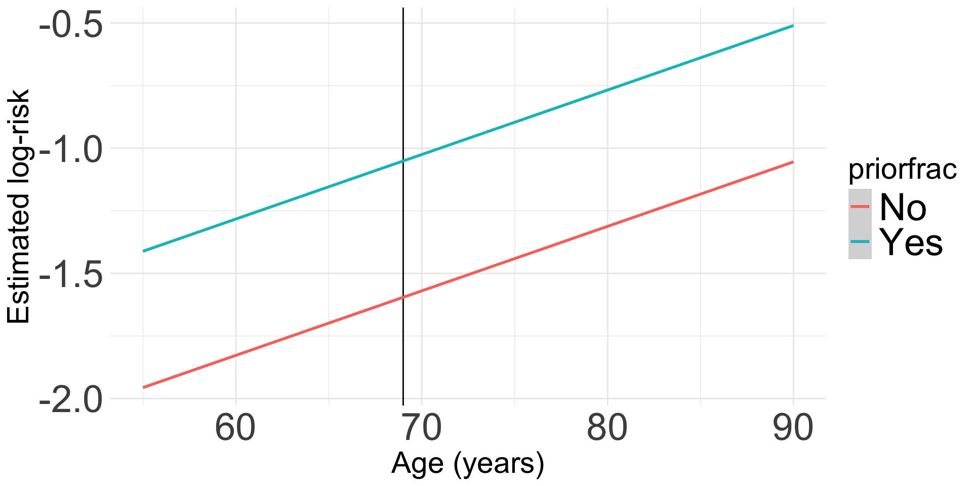
Visualization of interaction: We can look at the log-risk

  • This will help us understand the model that we fit
  • Ultimately, we do not need a visualization of the risk ratio because the main effects model is constant across age
Table of coefficient estimates
tidy(glow2_log_binom) %>% 
  gt() %>% 
  tab_options(table.font.size = 30) %>%
  fmt_number(decimals = 3)
term estimate std.error statistic p.value
(Intercept) −1.596 0.104 −15.414 0.000
priorfracYes 0.576 0.170 3.382 0.001
age_c 0.037 0.026 1.440 0.150
interaction_PF_age −0.009 0.017 −0.546 0.585
Code to make the following plot
prior_age = expand_grid(priorfrac = c("No", "Yes"), age_c = (55:90)-69) %>%
            mutate(interaction_PF_age = ifelse(priorfrac=="Yes", 1, 0)*age_c)
frac_pred_lb = predict(glow2_log_binom, prior_age, se.fit = F, type="link")
pred_glow_lb = prior_age %>% mutate(frac_pred = frac_pred_lb, 
                                  age = age_c + mean_age)

ggplot(pred_glow_lb) +
  geom_vline(xintercept = 69) +
  geom_smooth(method = "loess", aes(x = age, y = frac_pred, color = priorfrac)) +
  theme(text = element_text(size=35), title = element_text(size=22)) +
  labs(x = "Age (years)", y = "Estimated log-risk")

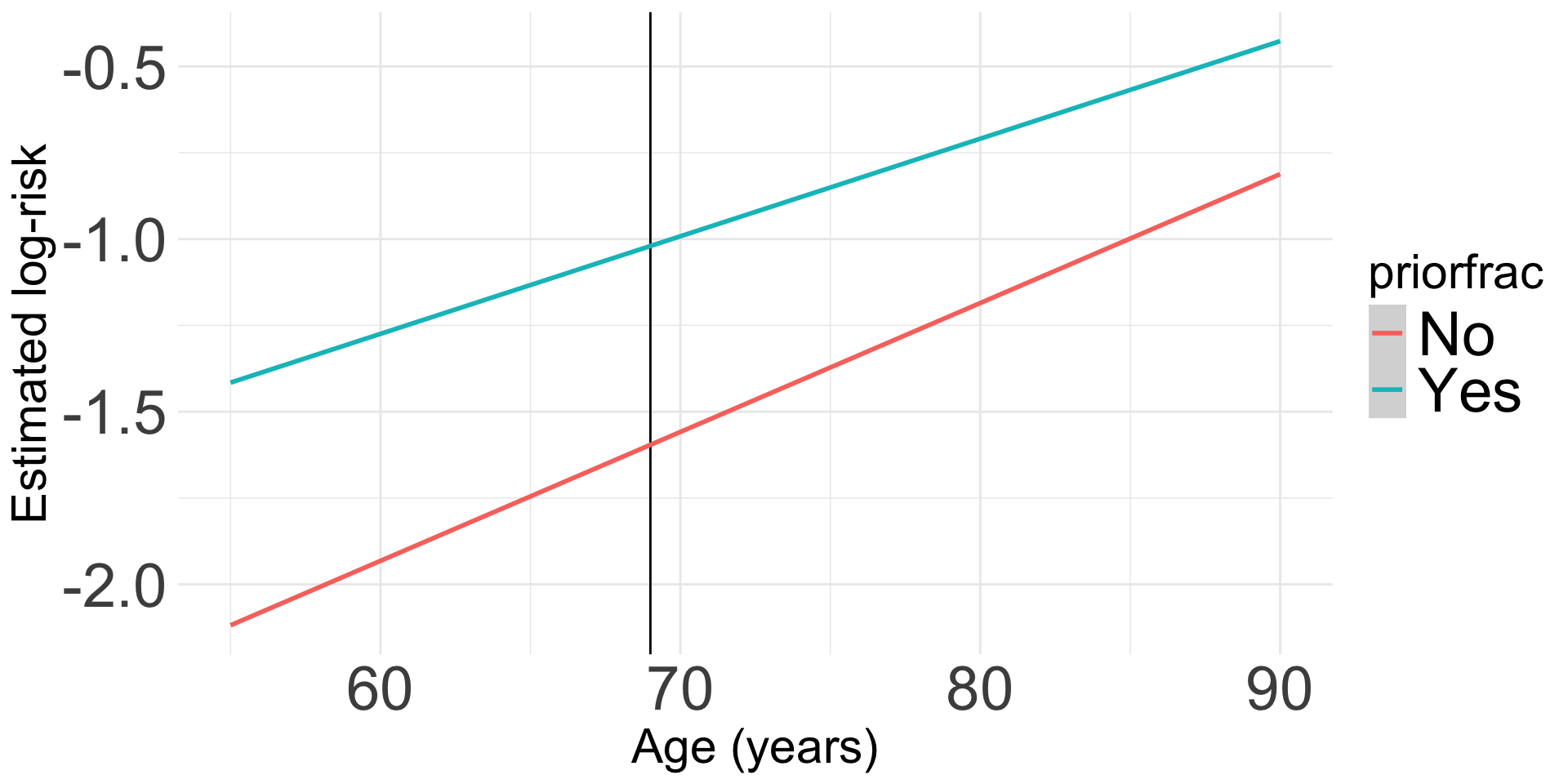
Predicted probabilities and visualizations

  • Does this look familiar?? It should!
    • The predicted probabilities from the logistic regression and the log-binomial regression should be the same!
Code to make the following plot
prior_age = expand_grid(priorfrac = c("No", "Yes"), age_c = (55:90)-69)
frac_pred_lb = predict(glow_log_binom, prior_age, se.fit = T, type="response")
pred_glow_lb = prior_age %>% mutate(frac_pred = frac_pred_lb$fit, 
                                  age = age_c + mean_age)

ggplot(pred_glow_lb) + #geom_point(aes(x = age, y = frac_pred, color = priorfrac)) +
  geom_smooth(method = "loess", aes(x = age, y = frac_pred, color = priorfrac)) +
  theme(text = element_text(size=20), title = element_text(size=16)) + ylim(0,1) +
  labs(color = "Prior Fracture", x = "Age (years)", y = "Predicted Probability of Fracture")

Final words on log-binomial vs logistic

  • Log-binomial is more common in field of Epidemiology


  • I prefer to use logistic regression because it is more stable AND I can calculate risk ratio from my odds ratio and predicted probability


  • If you use \(OR \approx RR\), then logistic regression will over-estimate the RR
    • BUT you can still use logistic regression to calculate the RR
    • Find the predicted probabilities for two groups you are comparing and then calculate the RR

More resources