Poster Info and Help

Nicky Wakim

2025-06-04

Some notes from last quarter’s posters (1/2)

Can you all see my feedback from last quarter? Let me know if you cannot, but want to
In methods, there is a difference between coding procedure and statistical procedure
- Example of something we do NOT report: If we get a dataset where the categorical variables (with worded categories) are represented as integers, then we convert the integers to the categories.
  - This is a coding procedure that automatically needs to be done to represent the variable accurately.
  - This is NOT a statistics procedure and we don’t report it. We’re not “converting” a continuous variable to a categorical one. We are performing data management to make sure the data code represent the data.
In conclusion/discussion, many people mentioned limitations but not how they affect the results
- Or made a wrong conclusion about the consequences
- See me to double check!!
“Data” is a plural word!
- Use like “Data are represented in Table…”

Some notes from last quarter’s posters (2/2)

Results
- No need to interpret the intercept unless you have an interaction
- If purposeful model selection, do NOT skip the odds ratios interpretations!!
- If you are limiting your Regression table to only the main variable, you need to explicitly state that this is from the final model and adjusted for other variables
There was A LOT of talk about generalizability being an issue because of the spread of our data
- Sample sistribution ALONE does not mean our results are not generalizable
- The more important question is: Are there enough people (in counts) in each group/demographic/etc to make a decent estimate?
Be really careful around language!!
- Using Why or How in your title is a little misleading – we can only answer “does”
- Make sure you do not make implications that we are uncovering a causal pathway!!
  - We are not!
  - The study design does NOT support this!

Things you can assume and not assume from your reader

Things people assume you are doing (correctly) and you do not need to share with an audience
- Following a codebook’s categories
- How you ran a certain model (aka don’t need to say we used glm() to fit the logistic regression model)
- You can assume people can read mathematical equations
- How age is calculated

Things you cannot assume people know
- How to read R code: do not include your model equation as an glm() function

Some notes

I will NOT be counting exact bullet points
- If it says 2-3, anything less than 4 is okay
- If it says 5-6, it shouldn’t be 1 and it shouldn’t be >10
Do NOT make bullet points really long!
- This was a big issue in last quarter’s poster
- Work to make things concise!! You are likely including too much information
I tried the QMD poster, and it is REALLY hard to troubleshoot
- I highly suggest making your poster in powerpoint!

Background

Length: 5-8 bullets
Purpose: Introduce the research question and why it is important to study
This section is non-technical.
- By reading just the introduction and conclusion, someone without a technical background should have an idea of what they study was about, why it is important, and what the main results are
You may start with your bullets from Lab 1, but you should edit it and make sure it flows into your report well!
Should contain some references

Methods

Length: 8-10 bullets
Purpose: Describe the analyses that were conducted and methods used to select variables and check diagnostics
Some important methods to discuss (You may divide these into your sections, not necessarily with these names)
- General approach to the dataset
- Variables and variable creation
- Model building: we performed purposeful selection
- Final model
- Model diagnostics

Methods example-ish

Data were collected from _____ in ____ year
We performed a complete case analysis on _____
We generated categorized variables for CO2 emissions and income levels
- CO2 emissions used quartiles
- Income levels used the specified groupings by Gapminder
We used purposeful model selection, a combination of field expertise and statistical methods, to determine the final model
Our final model included our outcome, life expectancy, with a main effect for female literacy rate while adjusting for confounders
- We adjusted for: CO2 emissions, income levels, world region, access to improved water, food supply, and intergovernmental groups
- We included an interaction between ____ and ____
We investigated model assumptions and diagnostics using ______
We used R version 4.4.1 to analyze data

Results: What should be in your results?

If you did purposeful model selection:

Table 1
Table showing odds ratios for your main variable + variable from interaction
One additional figure or table to understand your research question
Interpretations of odds ratios from Table in #2

If you did LASSO:

Table 1
Table or plot showing most important variables
One additional figure or table to help understand your question
Interpretations of important variables: identify top 1-3 that predict outcome

1. Table 1 (table summary in Lesson 2)

library(gtsummary)

gapm2_vars = gapm2 %>% 
  select(
    CO2emissions, 
    FoodSupplykcPPD, 
    FemaleLiteracyRate, 
    WaterSourcePrct, 
    four_regions, 
    members_oecd_g77, 
    income_levels1
  )

table1 = tbl_summary(
  gapm2_vars, 
  label = list(
    FemaleLiteracyRate = "Female literacy rate (%)", 
    CO2emissions = "CO2 emissions quartiles", 
    income_levels1 = "Income levels", 
    four_regions = "World region",
    WaterSourcePrct = "Access to improved water (%)",
    FoodSupplykcPPD = "Food supply (kcal PPD)",
    members_oecd_g77 = "Intergovernmental group"
    ),
  statistic = list(all_continuous() ~ "{mean} ({sd})")
  )

table1

Characteristic	N = 72¹
CO2 emissions quartiles	4.1 (5.6)
Food supply (kcal PPD)	2,812 (407)
Female literacy rate (%)	82 (23)
Access to improved water (%)	86 (16)
World region
Africa	20 (28%)
Americas	12 (17%)
Asia	17 (24%)
Europe	23 (32%)
Intergovernmental group
Group of 77	47 (65%)
OECD	7 (9.7%)
Others	18 (25%)
Income levels
Low income	10 (14%)
Lower middle income	24 (33%)
Upper middle income	24 (33%)
High income	14 (19%)
¹ Mean (SD); n (%)

2. Regression table or Forest plot (if no interactions)

reg_table = tbl_regression(
  final_model, 
  label = list(
    FemaleLiteracyRate ~ "Female literacy rate (%)", 
    CO2_q ~ "CO2 emissions quartiles", 
    income_levels1 ~ "Income levels", 
    four_regions ~ "World region",
    WaterSourcePrct ~ "Access to improved water (%)",
    FoodSupplykcPPD ~ "Food supply (kcal PPD)",
    members_oecd_g77 ~ "Intergovernmental group"
    )) %>%   
  as_gt() %>% 
  tab_options(table.font.size = 20) %>%
  cols_width(label ~ px(250))
reg_table

Characteristic	Beta	95% CI¹	p-value
Female literacy rate (%)	-0.07	-0.17, 0.02	0.13
CO2 emissions quartiles
Quartile 1	—	—
Quartile 2	1.1	-2.7, 4.9	0.6
Quartile 3	-0.29	-5.1, 4.6	>0.9
Quartile 4	-0.60	-5.6, 4.5	0.8
Income levels
Low income	—	—
Lower middle income	5.4	0.75, 10	0.024
Upper middle income	6.1	0.20, 12	0.043
High income	8.0	1.4, 15	0.018
World region
Africa	—	—
Americas	9.0	4.9, 13	<0.001
Asia	5.3	2.0, 8.5	0.002
Europe	6.9	1.1, 13	0.020
Access to improved water (%)	0.17	0.03, 0.30	0.015
Food supply (kcal PPD)	0.00	0.00, 0.01	0.073
Intergovernmental group
Group of 77	—	—
OECD	1.1	-4.2, 6.5	0.7
Others	1.0	-4.0, 6.1	0.7
¹ CI = Confidence Interval

2. Regression table or Forest plot (if no interactions)

library(broom.helpers)
model_tidy = tidy_and_attach(final_model, conf.int=T) %>%
  tidy_remove_intercept() %>%
  tidy_add_reference_rows() %>% tidy_add_estimate_to_reference_rows() %>%
  tidy_add_term_labels() %>%
  mutate(var_label = case_match(var_label, 
                               "Female literacy rate (%)" ~ "", 
                               "Food supply (kcal PPD)" ~ " ", 
                               "Access to improved water (%)" ~ "   ", 
                               "CO2 emissions quartiles" ~ "CO2 emissions \n quartiles", 
                               "Income levels" ~ "Income levels", 
                               "Intergovernmental group" ~ "Intergovern- \n mental group", 
                               .default = var_label
                         ))

forest_plot = ggplot(data=model_tidy, aes(y=label, x=estimate, xmin=conf.low, xmax=conf.high)) + 
  facet_grid(rows = vars(var_label), scales = "free",
             space='free_y', switch = "y") + 
  geom_point(size = 3) +  geom_errorbarh(height=.2) + 
  geom_vline(xintercept=0, color='#C2352F', linetype='dashed', alpha=1) +
  theme_classic() +
  labs(x = "Beta", y = "Variables") +
  theme(axis.title = element_text(size = 20), axis.text = element_text(size = 20), 
        title = element_text(size = 20), strip.placement = "outside", 
        strip.text.y.left = element_text(size = 18, angle = 0), 
        strip.background = element_blank())

2. Regression table or Forest plot (if no interactions)

This is a fun one to investigate!
Stick to the regression table if you are having trouble with this!

library(broom.helpers)

model_tidy = tidy_and_attach(final_model, conf.int=T) %>%
  tidy_remove_intercept() %>%
  tidy_add_reference_rows() %>% tidy_add_estimate_to_reference_rows() %>%
  tidy_add_term_labels() %>%
  mutate(var_label = case_match(var_label, 
                               "Female literacy rate (%)" ~ "", 
                               "Food supply (kcal PPD)" ~ " ", 
                               "Access to improved water (%)" ~ "   ", 
                               "CO2 emissions quartiles" ~ "CO2 emissions \n quartiles", 
                               "Income levels" ~ "Income levels", 
                               "Intergovernmental group" ~ "Intergovern- \n mental group", 
                               .default = var_label
                         ))

forest_plot = ggplot(data=model_tidy, aes(y=label, x=estimate, xmin=conf.low, xmax=conf.high)) + 
  facet_grid(rows = vars(var_label), scales = "free",
             space='free_y', switch = "y") + 
  geom_point(size = 3) +  geom_errorbarh(height=.2) + 
  geom_vline(xintercept=0, color='#C2352F', linetype='dashed', alpha=1) +
  theme_classic() +
  labs(x = "Beta", y = "Variables") +
  theme(axis.title = element_text(size = 20), axis.text = element_text(size = 20), 
        title = element_text(size = 20), strip.placement = "outside", 
        strip.text.y.left = element_text(size = 18, angle = 0), 
        strip.background = element_blank())
forest_plot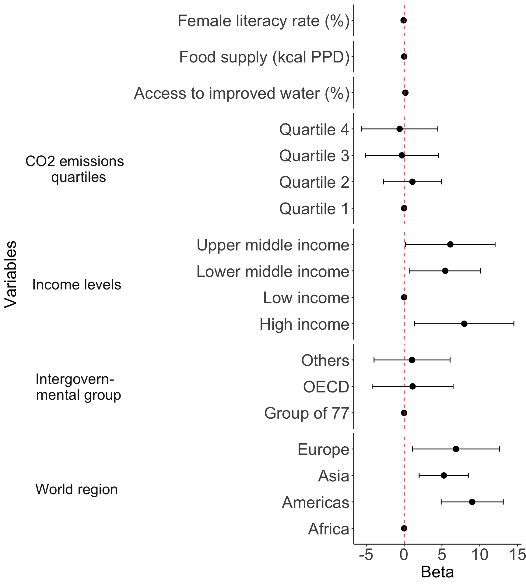

Important note if you have interactions

Please check your Quiz 3 feedback!
- Many of you are not quite interpreting interactions correctly
There is extra care to reporting results from interactions
Please make sure you use estimable() to get the correct effects!
- If you have an interaction with a categorical variable, then your main variable’s “effect” should be reported for each category
See HW 3 and Lecture 10 for reporting!
You will NOT include the adjusting variables in the table/plot
- But you need to say adjusting for all other variables in model from methods

Table/plot if you have interactions!!

Let’s say my model from HW 3 included other variables and my main research question is about association between death and if infection is probable at ICU intake

Table __: Estimated odds ratios and confidence intervals of death at discharge. Odds ratios are comparing infection probable and not probable at ICU intake depending for two cases when cancer is and is not part of problem. Odds ratios adjust for all other variable in the model presented in methods.

Cancer	Infection	Estimated OR	95% CI
Cancer part of present problem	Infection probable at ICU intake
	No
	Yes	FILL HERE	FILL HERE
Cancer not part of present problem	Infection probable at ICU intake
	No
	Yes	FILL HERE	FILL HERE

Saving tables

For tables: gtsave in the gt package should work!
For figures/plots: ggsave in the ggplot2 package should work!

gtsave(reg_table, filename = here("lessons/19_Poster_help/reg_table.png"))
gtsave(table1, filename = here("lessons/19_Poster_help/table1.png"))
ggsave(forest_plot, filename = here("lessons/19_Poster_help/forest_plot.png"))

When I first ran the above, I got the following message: The package "webshot2" is required to save gt tables as images. ✖ Would you like to install it? 1: Yes 2: No
- I inputted 1

Poster Info and Help

Some notes from last quarter’s posters (1/2)

Some notes from last quarter’s posters (2/2)

Things you can assume and not assume from your reader

Some notes

Background

Methods

Methods example-ish

Results: What should be in your results?

1. Table 1 (table summary in Lesson 2)

2. Regression table or Forest plot (if no interactions)

2. Regression table or Forest plot (if no interactions)

2. Regression table or Forest plot (if no interactions)

Important note if you have interactions

Table/plot if you have interactions!!

Saving tables

Any other questions about the poster?