Lab 3: Feedback and Discussion

Nicky Wakim

2025-05-12

Lab 3 Feedback

Some fo you did main covariate + 4 other variables and some did main covariate + 5 other variables
- Okay either way
In presentation of odds ratios (forest plot and tables), it’s important to include the reference group
- Gives the reader context for the comparison

Get into groups of 2-4

No more than 4!
Introduce yourself and your research question
Share you html documents with each other (email, airdrop, etc.)

05:00

Help with forest plot: ordering categories

source("/Users/wakim/Library/CloudStorage/OneDrive-OregonHealth&ScienceUniversity/Projects/Teaching_DEIJ_Datasets/Datasets/Food_insecurity/Code/Labs/Lab_02_work.R")

Let’s say I ran this model:

model = wbns4 %>% 
  glm(formula = FOOD_INSEC ~ PPINCIMP + XACSNET + FAMSIZE, family = binomial)

Help with forest plot: ordering categories

library(broom.helpers)
MLR_tidy0 = tidy_and_attach(model,  conf.int=T, exponentiate = T) %>%
  tidy_remove_intercept() %>%
  tidy_add_reference_rows() %>%
  tidy_add_estimate_to_reference_rows() %>%
  tidy_add_term_labels()

glimpse(MLR_tidy0)

Rows: 31
Columns: 16
$ term           <chr> "PPINCIMP$10,000 to $12,499", "PPINCIMP$100,000 to $124…
$ variable       <chr> "PPINCIMP", "PPINCIMP", "PPINCIMP", "PPINCIMP", "PPINCI…
$ var_label      <chr> "PPINCIMP", "PPINCIMP", "PPINCIMP", "PPINCIMP", "PPINCI…
$ var_class      <chr> "factor", "factor", "factor", "factor", "factor", "fact…
$ var_type       <chr> "categorical", "categorical", "categorical", "categoric…
$ var_nlevels    <int> 21, 21, 21, 21, 21, 21, 21, 21, 21, 21, 21, 21, 21, 21,…
$ contrasts      <chr> "contr.treatment", "contr.treatment", "contr.treatment"…
$ contrasts_type <chr> "treatment", "treatment", "treatment", "treatment", "tr…
$ reference_row  <lgl> TRUE, FALSE, FALSE, FALSE, FALSE, FALSE, FALSE, FALSE, …
$ label          <chr> "$10,000 to $12,499", "$100,000 to $124,999", "$12,500 …
$ estimate       <dbl> 1.000000000, 0.060863278, 0.873493696, 0.043281443, 0.8…
$ std.error      <dbl> NA, 0.2175317, 0.1557261, 0.2940413, 0.1432175, 0.25032…
$ statistic      <dbl> NA, -12.8676662, -0.8685401, -10.6788784, -1.1890139, -…
$ p.value        <dbl> NA, 6.843892e-38, 3.850987e-01, 1.278065e-26, 2.344342e…
$ conf.low       <dbl> NA, 0.0390983422, 0.6433397149, 0.0233193469, 0.6368560…
$ conf.high      <dbl> NA, 0.09195374, 1.18491604, 0.07444924, 1.11676827, 0.1…

Help with forest plot: ordering categories

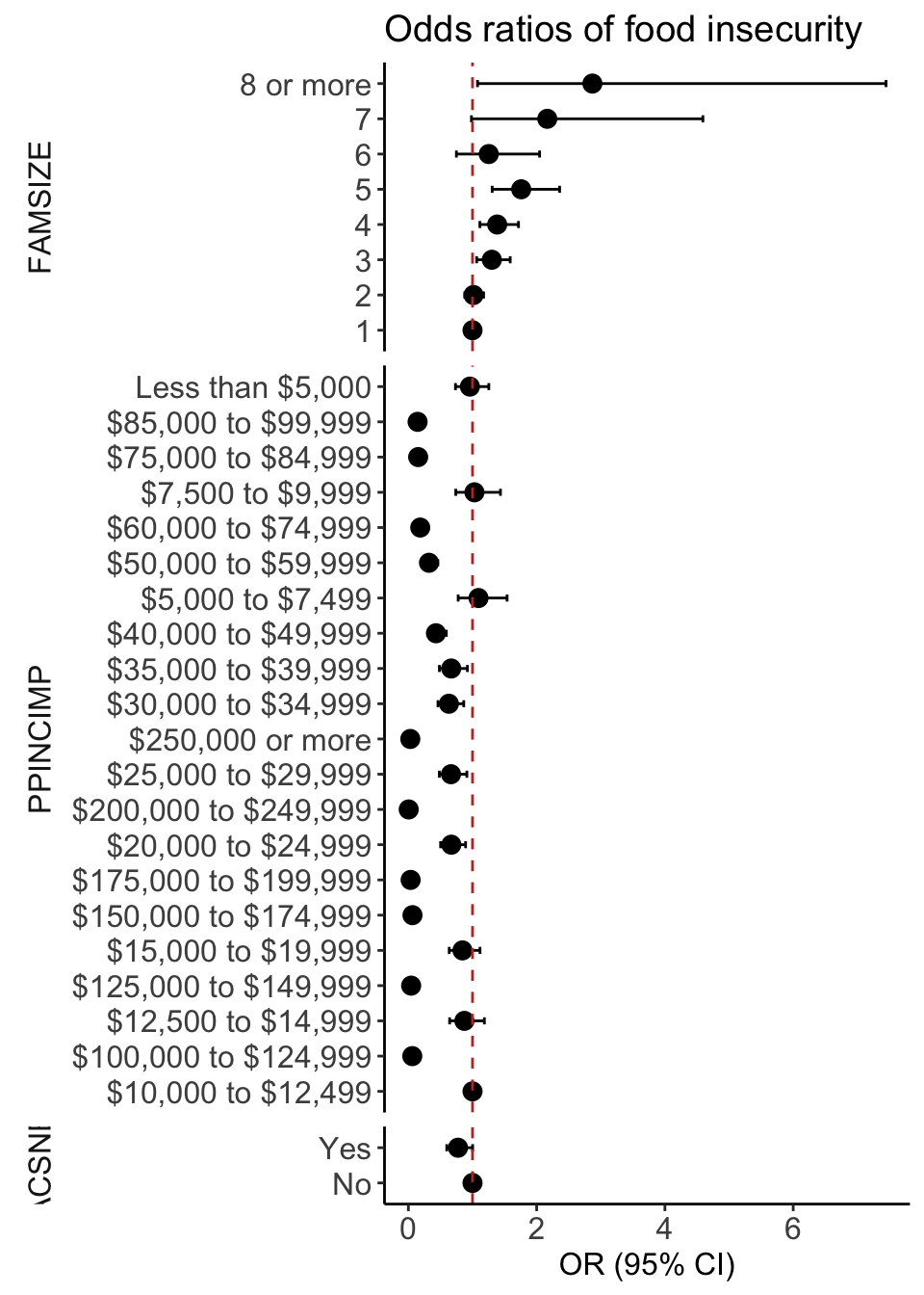
plot_MLR0 = ggplot(data=MLR_tidy0, 
       aes(y=label, x=estimate, xmin=conf.low, xmax=conf.high)) + 
  geom_point(size = 3) +  geom_errorbarh(height=.2) + 
  
  geom_vline(xintercept=1, color='#C2352F', linetype='dashed', alpha=1) +
  theme_classic() +
  
  facet_grid(rows = vars(var_label), scales = "free",
             space='free_y', switch = "y") + 
  
  labs(x = "OR (95% CI)", 
       title = "Odds ratios of food insecurity") +
  theme(axis.title = element_text(size = 12), 
        axis.text = element_text(size = 12), 
        title = element_text(size = 12), 
        axis.title.y=element_blank(), 
        strip.text = element_text(size = 12), 
        strip.placement = "outside", 
        strip.background = element_blank())

Help with forest plot: ordering categories

plot_MLR0

Help with forest plot: ordering categories

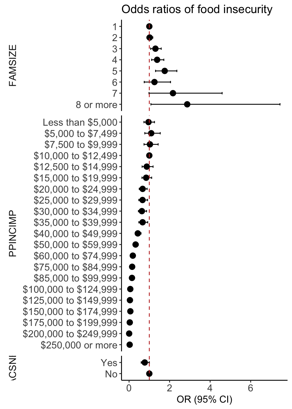
MLR_tidy = MLR_tidy0  %>%
              mutate(order = case_match(label, 
                            "Less than $5,000" ~ 1, 
                            "$5,000 to $7,499" ~ 2, 
                            "$7,500 to $9,999" ~ 3, 
                            "$10,000 to $12,499" ~ 4, 
                            "$12,500 to $14,999" ~ 5, 
                            "$15,000 to $19,999" ~ 6, 
                            "$20,000 to $24,999" ~ 7, 
                            "$25,000 to $29,999" ~ 8, 
                            "$30,000 to $34,999" ~ 9, 
                            "$35,000 to $39,999" ~ 10, 
                            "$40,000 to $49,999" ~ 11, 
                            "$50,000 to $59,999" ~ 12, 
                            "$60,000 to $74,999" ~ 13, 
                            "$75,000 to $84,999" ~ 14, 
                            "$85,000 to $99,999" ~ 15, 
                            "$100,000 to $124,999" ~ 16, 
                            "$125,000 to $149,999" ~ 17, 
                            "$150,000 to $174,999" ~ 18, 
                            "$175,000 to $199,999" ~ 19, 
                            "$200,000 to $249,999" ~ 20, 
                            "$250,000 or more" ~ 21, 
                            "1" ~ 1, 
                            "2" ~ 2, 
                            "3" ~ 3, 
                            "4" ~ 4, 
                            "5" ~ 5, 
                            "6" ~ 6, 
                            "7" ~ 7, 
                            "8 or more" ~ 8,
                            .default = 0)) %>%
            mutate(label = fct_reorder(label, desc(order)))

Help with forest plot: ordering categories

plot_MLR = ggplot(data=MLR_tidy, 
       aes(y=label, x=estimate, xmin=conf.low, xmax=conf.high)) + 
  geom_point(size = 3) +  geom_errorbarh(height=.2) + 
  
  geom_vline(xintercept=1, color='#C2352F', linetype='dashed', alpha=1) +
  theme_classic() +
  
  facet_grid(rows = vars(var_label), scales = "free",
             space='free_y', switch = "y") + 
  
  labs(x = "OR (95% CI)", 
       title = "Odds ratios of food insecurity") +
  theme(axis.title = element_text(size = 12), 
        axis.text = element_text(size = 12), 
        title = element_text(size = 12), 
        axis.title.y=element_blank(), 
        strip.text = element_text(size = 12), 
        strip.placement = "outside", 
        strip.background = element_blank())

Help with forest plot: ordering categories

plot_MLR

Questions to consider

How did you handle any categorical variables?
- Income, family size, number of children, etc
Are the categories for the forest plot in order?
How did you interpret your estimated odds ratios?
- If you have many categories in your main variable, do you see a trend?
- What might be a better way to report a trend?
If you had interactions, how would your interpretation change?