Lesson 1: Introduction to Probability

Nicky Wakim

2025-09-29

Learning Objectives

Define key probability and its relationship to randomness.
Use simple simulations (e.g., coin flips in R) to illustrate randomness in equally likely outcomes.
Identify sample spaces and events for basic experiments, and define probability calculations.

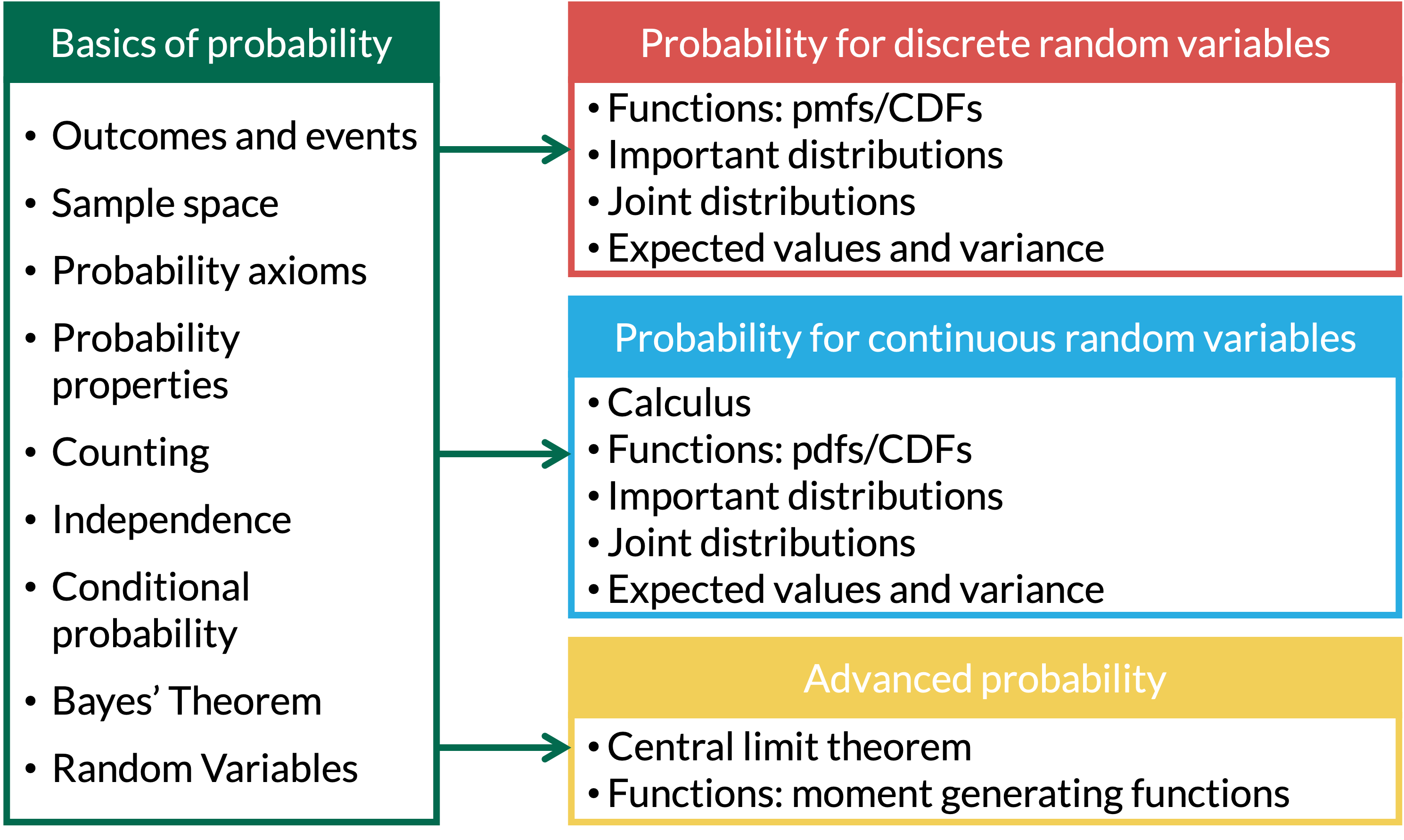
Where are we?

Learning Objectives

Define key probability and its relationship to randomness.

Use simple simulations (e.g., coin flips in R) to illustrate randomness in equally likely outcomes.
Identify sample spaces and events for basic experiments, and define probability calculations.

What is probability? (1/2)

We hear the word “probability” pretty often
- Common in news reports, advertisements, sports, medicine, etc.

Researchers say the probability of living past 110 is on the rise

CNBC, 2021

We may hear “probability” or similar words like “chance,” “likelihood,” or “odds”

Scientists fine-tune odds of asteroid Bennu hitting Earth through 2300 with NASA probe’s help

Space.com, 2021

Before we take one more step

The following few slides use some undefined words to define new words that in turn define other words
It’s confusing!
We’re going off assumption that we all have some understanding of probability, so stop me if you are confused!

Learning Objectives

Define key probability and its relationship to randomness.

Use simple simulations (e.g., coin flips in R) to illustrate randomness in equally likely outcomes.

Identify sample spaces and events for basic experiments, and define probability calculations.

Probability and randomness

Probability requires randomness
Something is random if there are many potential outcomes, but there is uncertainty which outcome will occur

Outcomes can be “equally likely,” meaning each outcome has the same probability of happening
- But random does NOT necessarily mean equally likely
We often use physical randomness to demonstrate equally likely outcomes
- Think: flipping coins, rolling a dice, drawing cards

The occurrence of outcomes can be uncertain, but there is an underlying distribution of the probability of outcomes
- There is a distribution of outcomes over large number of (hypothetical repetitions)

A single coin flip then 100 coin flips

Seeing Theory, Chapter 1: Basic Probability, Chance Events

How do we simulate this in R?

We know that heads and tails are equally likely for a single flip

set.seed(13)
coin = c("heads", "tails")
sample(coin, 1)

[1] "tails"

When we only flip the coin once, we only only get one outcome (heads or tails)
- We cannot see any distribution of the probability of outcomes

What if I sample 10 coin flips?

How many tails do we get? Are we getting closer to a distribution of heads and tails that we expect?

Results and running proportion of H for 10 flips of a fair coin.
Flip	Result	Running count of H	Running proportion of H
1	H	1	1.000
2	T	1	0.500
3	H	2	0.667
4	T	2	0.500
5	H	3	0.600
6	T	3	0.500
7	T	3	0.429
8	T	3	0.375
9	T	3	0.333
10	T	3	0.300

What if I sample 100 coin flips?

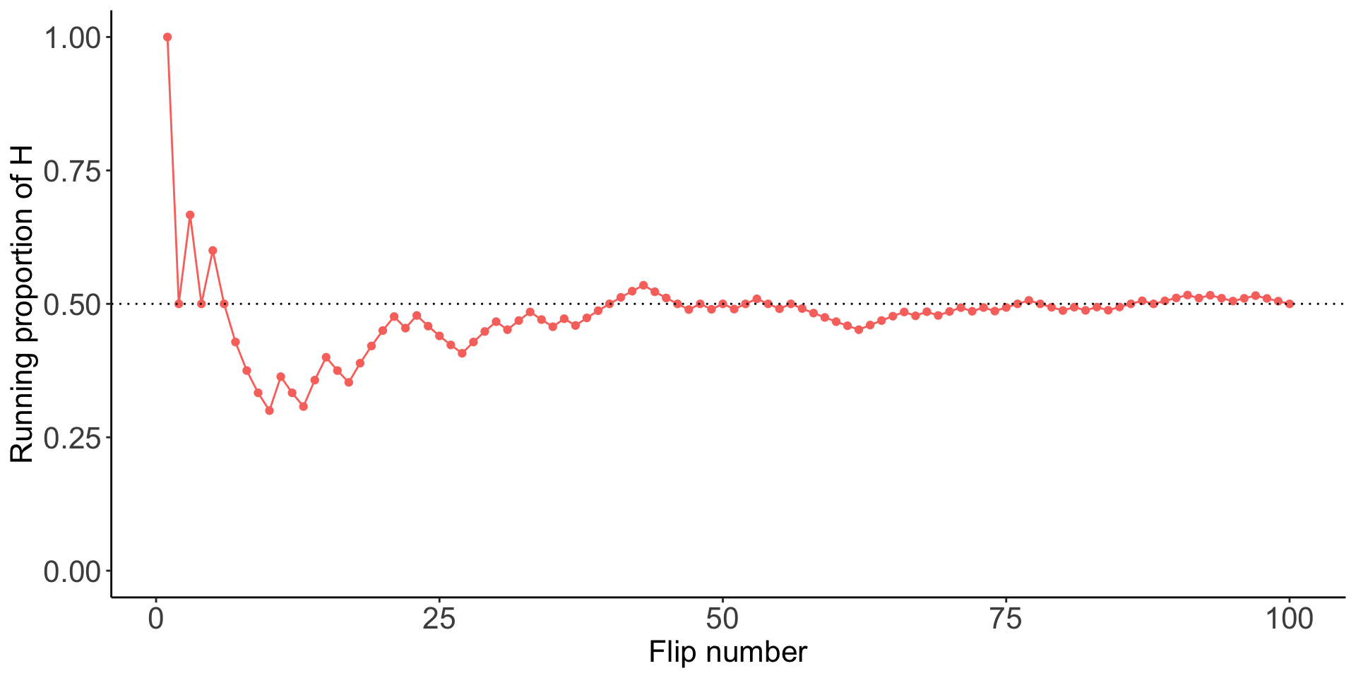
What’s the point?

We know the probability of a heads is 0.5!
Why do we need to simulate 100s or 1000s of coin flips?
With enough repetitions, we can use simulations to approximate the probability of an event
Simulations involve artificial recreation of a random phenomenon

Why are simulations important? (bigger picture)

In the previous example, coding a simulation seemed more educational than necessary
We can often calculate probabilities mathematically, but we will eventually get to complex calculations
- Simulations can help us (or be necessary) to solve a problem when calculations are complex
Simulations are a great way to check your work!
Simulation based reasoning is helpful in statistics
- You’ll see this in confidence intervals in Biostatistics courses
Simulations allow you to change assumptions easily and see how they affect your results
It is often how statisticians “run” experiments on their methods of hypotheses

Learning Objectives

Define key probability and its relationship to randomness.
Use simple simulations (e.g., coin flips in R) to illustrate randomness in equally likely outcomes.

Identify sample spaces and events for basic experiments, and define probability calculations.

Outcomes, events, sample spaces

Definition: Outcome

The possible results in a random phenomenon.

Definition: Sample Space

The sample space \(S\) is the set of all outcomes

Definition: Event

An event is a collection of some outcomes. An event can include multiple outcomes or no outcomes (a subset of the sample space).

When thinking about events, think about outcomes that you might be asking the probability of. For example, what is the probability that you get a heads or a tails in one flip? (Answer: 1)

Coin Toss Example: 1 coin (1/3)

Single coin toss

Suppose you toss one coin.

What are the possible outcomes?
What is the sample space?
What are the possible events?

Coin Toss Example: 1 coin (2/3)

Suppose you toss one coin.

What are the possible outcomes?
- Heads (\(H\))
- Tails (\(T\))

Note

When something happens at random, such as a coin toss, there are several possible outcomes, and exactly one of the outcomes will occur.

Coin Toss Example: 1 coin (3/3)

What is the sample space?
- \(S =\)

What are the possible events?

Note #1

We use curly brackets (\(\{\}\)) to denote a set (collecting a list of outcomes or values)

Note #2

The total number of possible events is \[2^{|S|}\] where \(|S|\) is the total number of outcomes in the sample space. Also, possible events are not necessarily something that can actually occur (i.e. getting a heads and a tails on a single coin flip)

Coin Toss Example: 2 coins

Suppose you toss two coins.

What is the sample space? Assume the coins are distinguishable
- \(S =\)

What are some possible events?
- \(A =\) exactly one \(H =\)
- \(B =\) at least one \(H =\)

More info on events and sample spaces

We usually use capital letters from the beginning of the alphabet to denote events. However, other letters might be chosen to be more descriptive.
- Examples: \(A, B, C, A_1, A_2\)
We can also define a new event as a combination of other events
- Examples: \(A \cup B\) (union), \(A \cap B\) (intersection), \(A^C\) (complement)

We use the notation \(|S|\) to denote the size of the sample space.

The total number of possible events is \(2^{|S|}\), which is the total number of possible subsets of \(S\).

The empty set, denoted by \(\emptyset\), is the set containing no outcomes.

Example: Keep sampling until…

Suppose you keep sampling people until you have someone with high blood pressure (BP)

What is the sample space?

Let \(H =\) denote someone with high BP.
Let \(H^C =\) denote someone with not high blood pressure, such as low or regular BP.

Then, \(S =\)

Let’s define probability with events and spaces

If \(S\) is a finite sample space, with equally likely outcomes, then

\[\mathbb{P}(A) = \frac{|A|}{|S|}\]

In human speak:

For equally likely outcomes, the probability that a certain event occurs is: the number of outcomes within the event of interest (\(|A|\)) divided by the total number of possible outcomes (\(|S|\))

\[\mathbb{P}(A) = \frac{\text{total number of outcomes in event A}}{\text{total number of outcomes in sample space}}\]

Thus, it is important to be able to count the outcomes within an event

A probability is a function…

\(\mathbb{P}(A)\) is a function with
- Input: event \(A\) from the sample space \(S\), (\(A \subseteq S\))
  - \(A \subseteq S\) means “A contained within S” or “A is a subset of S”
- Output: a number between 0 and 1 (inclusive)

The probability function maps an event (input) to value between 0 and 1 (output)
- When we speak of the probability function, we often call the values between 0 and 1 “probabilities”
  - Example: “The probability of drawing a heart is 0.25” for \(P(\text{heart}) = 0.25\)

The probability function needs to follow some specific rules (called axioms)!