Lesson 9: Cumulative distribution functions (CDFs)
2025-10-22
Where are we?
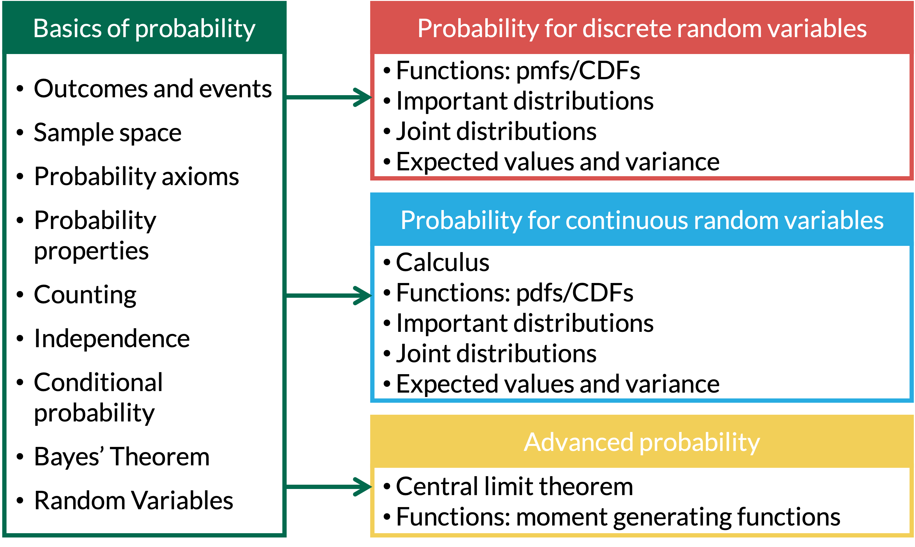
How to define CDFs for discrete and continuous RVs?
Discrete RV \(X\):
- pmf: \(p_X(x) = P(X=x)\)
- CDF: \(F_X(x) = P(X \leq x) = \sum\limits_{\{all\ y:\ y\leq x\}} p_X(y)\)
Continuous RV \(X\):
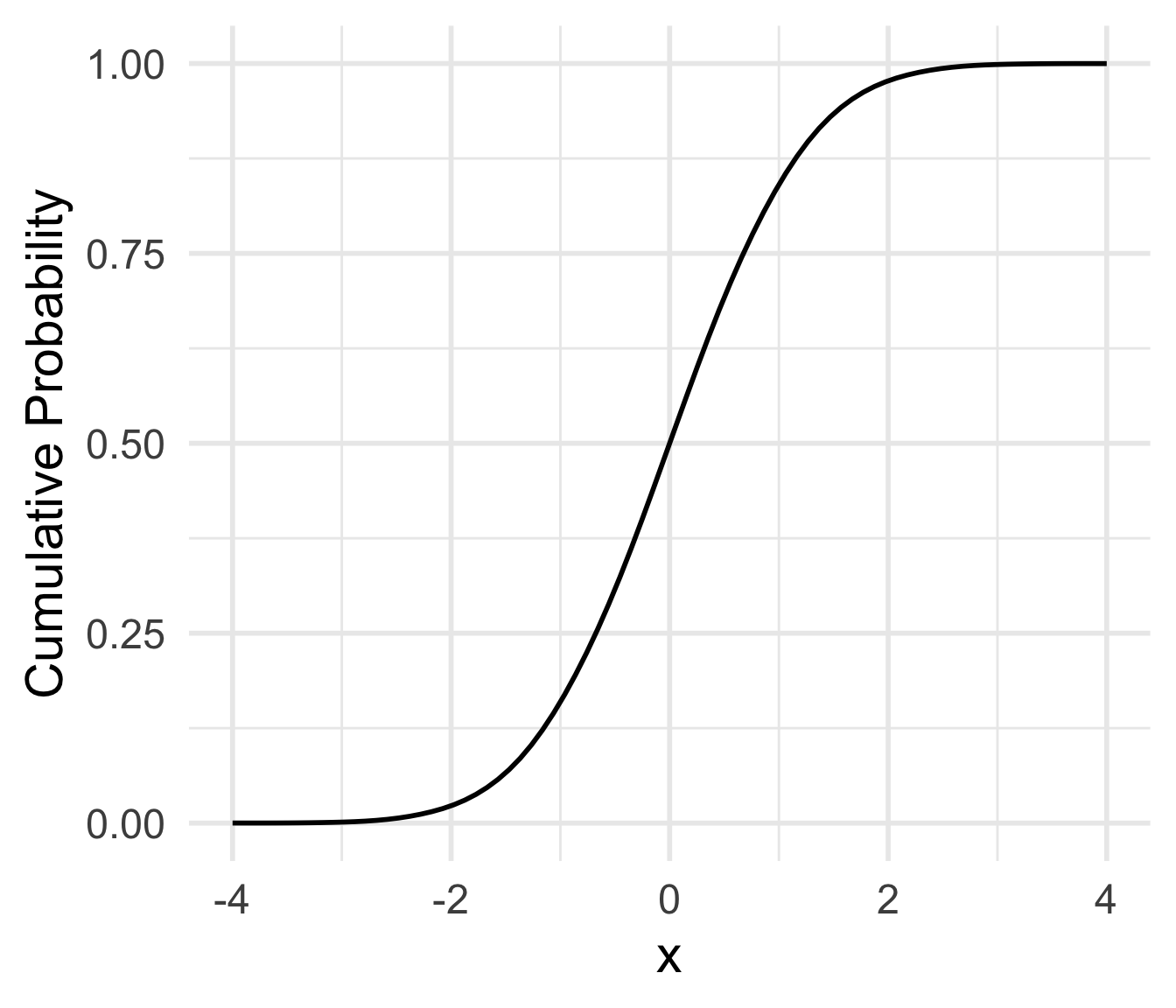
- density: \(f_X(x)\)
- probability: \(P(a \leq X \leq b) = \int_a^b f_X(x)dx\)
- CDF: \(F_X(x) = P(X \leq x) = \int_{-\infty}^x f_X(s)ds\)
Falls in Older Adults Revisited (4/5)
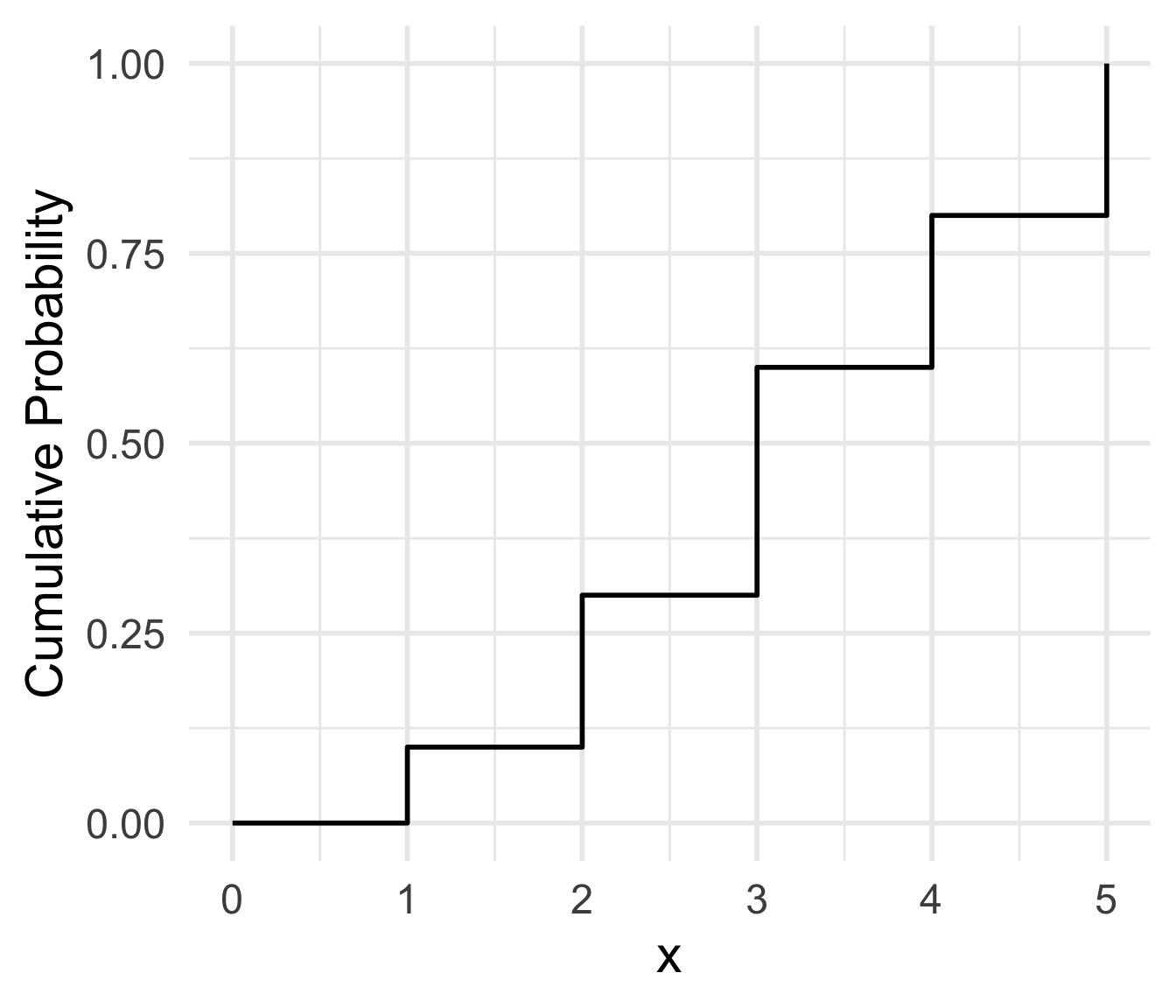
Example 1: Falls in Older Adults
- Plot the CDF of \(X\).
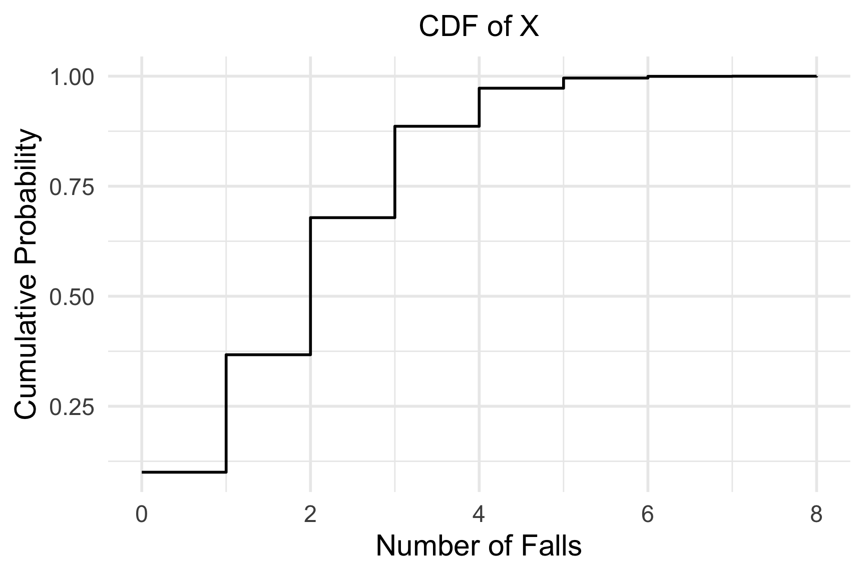
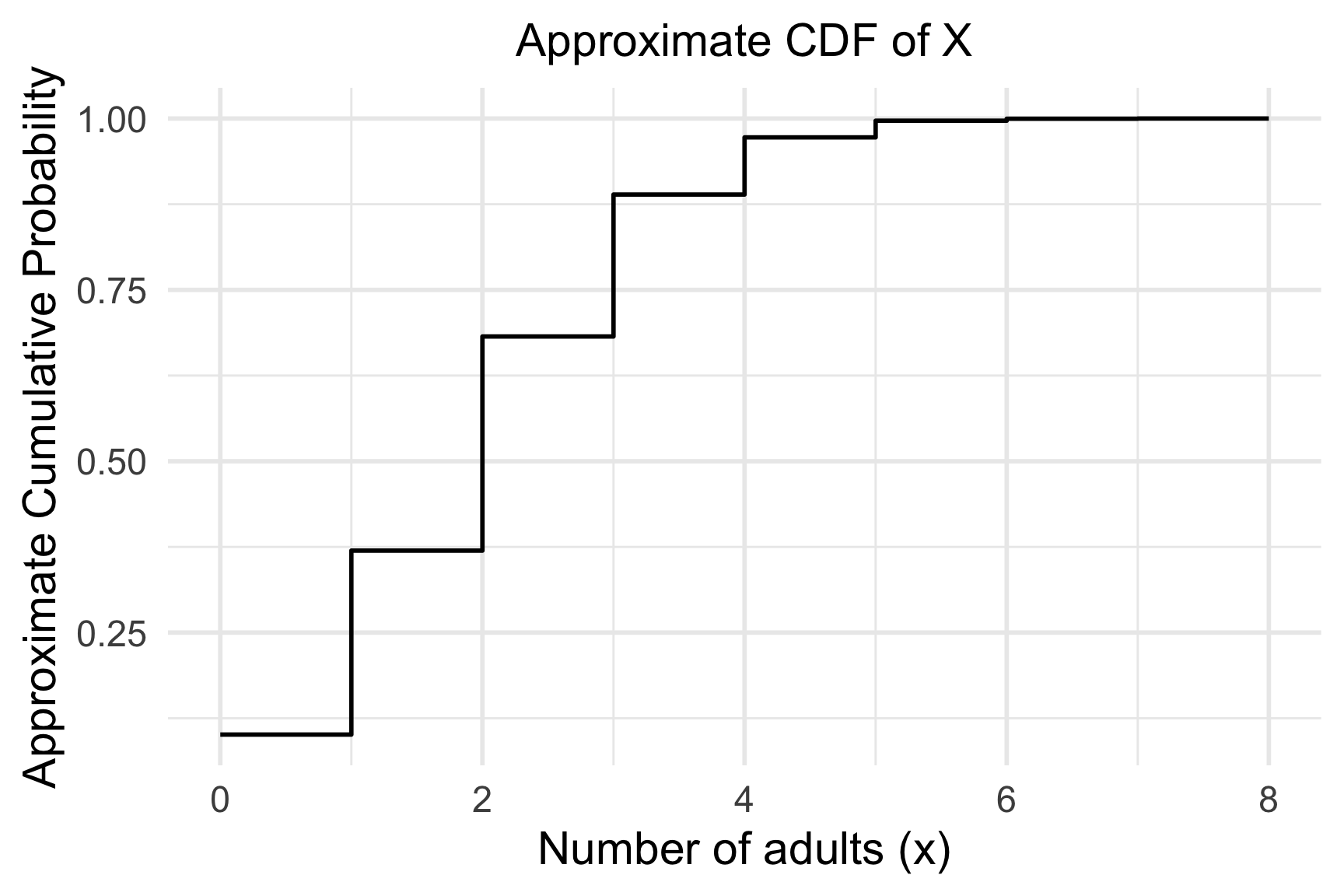
Falls in Older Adults Revisited (4/5)
Example 1: Falls in Older Adults
- Simulate \(X\) for 10000 groups and plot the approximated CDF.