Muddy Points

Modified

November 10, 2025

Fall 2025

1. Going through integration by parts again

Here’s a pretty good video on integration by parts!

Here’s the Calc review muddy points with a few words on integration by parts.

2. Maybe expand on why the “Expected Value” is sum/integral “x” times the pmf (for discrete) and pdf (for continuous)?

Think back to our discrete example with the die. Our expected value was the weighted average of all the possible outcomes (weighted by their probability). So our expected value for discrete RVs will always be that weighted average: \[\mathbb{E}[X] = \sum_{i=1}^n x_ip_X(x_i)\]

For continuous RVs, they can take infinite possible values, so we cannot sum across the pdf the same way. We still want the weighted average, so we need to find a way to “sum” the weighted outcomes for the continuous RV, which translates to an integral.

Here’s a fairly good explanation on StackExchange..)

3. Muddiest point may be the last example with making sure I get the bounds correct.

Final example: Let \(f_{X,Y}(x,y)= 2e^{-(x+y)}\), for \(0 \leq x \leq y\). Find \(\mathbb{E}[X]\).

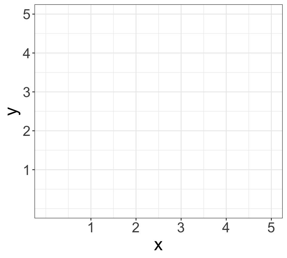
Let’s start with a plot for the domain. We have \(0 \leq x \leq y\), so we know that \(x\geq0\) and because \(y\geq x\), then \(y\geq0\), so we’ll have a plot of all positive values of \(x\) and \(y\):

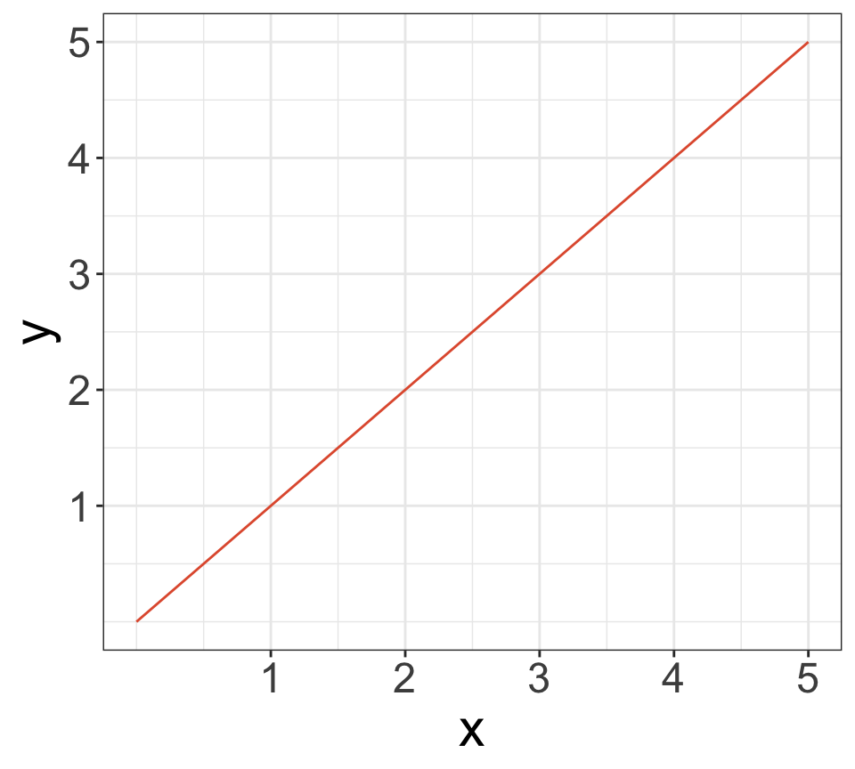
Okay, now let’s add the information that \(y \geq x\). We can look at the line, \(y=x\), and identify the area on the side of the line that upholds \(y \geq x\):

The area above the line is where \(y\geq x\):

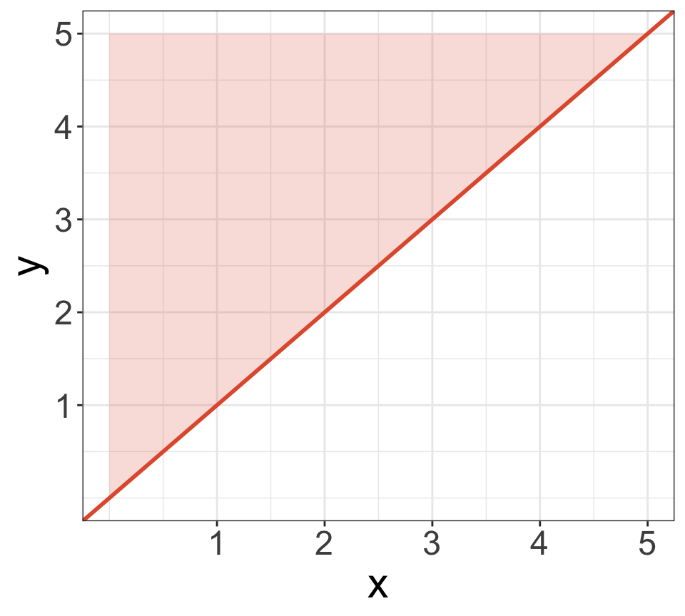
So we need to find the bounds for the orange region in terms of \(x\) and \(y\).

Whichever random variable is on the inner integral will need to incorporate the \(y=x\) line. If we integrate over \(y\) first, we will integrate from \(y=x\) to \(y=\infty\). Once we have incorporated the line into our first integral, then we no longer need to worry about the \(y=x\) line. For \(x\), we can integrate from \(x=0\) to \(x=\infty\).