Muddy Points
Lesson 14: Variance
Fall 2025
1. I don’t quite get why we occasionally choose to treat things as iid. Last class we talked about how the hotel prices could be $190 or $210, then in this class we decided they were all iid. That seems arbitrary to me.
You are right, the hotel room problem did not need the identical distributions in either class. I definitely mispoke by saying they were iid. Even though they have the same expected value and variance, they are not necessarily from the same distribution. They are independent, but not necessarily identically distributed. They all have the same variance, so I can still use \[\sum_{i=1}^{30} Var(X_i) = 30Var(X)\]
It was more that, last class, we did not specify the standard deviation. We could find the expected value of the total cost without knowing the standard deviation, and thus without necessarily assuming the cost of the hotel rooms were identical random variables. In this class, we needed the standard deviation for the cost of each hotel room. We could have made them different, but we made all of them $10.
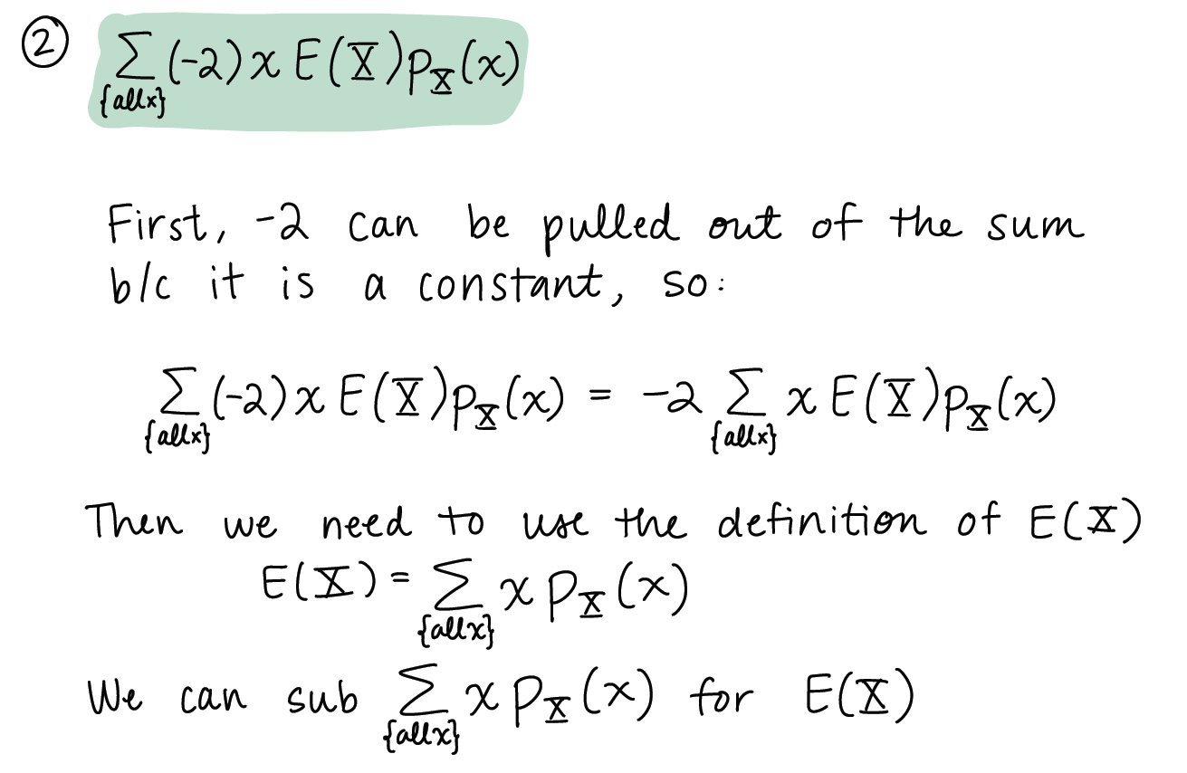
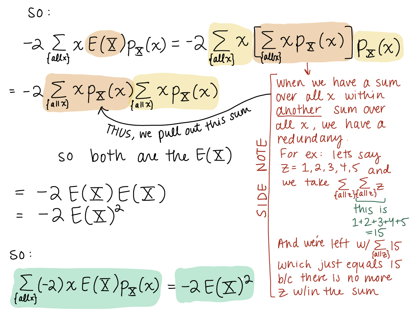
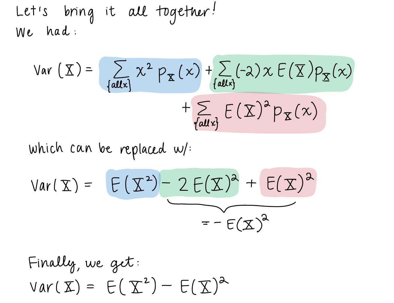
2. The math breakdown of $(X) = E[X^2] - E[X]^2 I’m not sure where the \(X\) value in the term 2 summation \(\mu_xXp_x(x)\) where did \(Xp_x(x)\) go?
I go through that breakdown in the first muddy point from Fall 2023 (below). Check out the term 2 part that is highlighted in green-ish.
3. I think what I am muddy on the difference between the Corollary 2 and Corollary 3, is the “n.” Where does the “n” come from in Corollary 3.
Here are the corollaries:
Corollary 2
For independent RV’s \(X_i\), \(i=1,2,\dots, n\), \[Var\Bigg(\sum_{i=1}^n X_i\Bigg) = \sum_{i=1}^n Var(X_i).\]
Corollary 3
For independent identically distributed (i.i.d.) RV’s \(X_i\), \(i=1,2,\dots, n\), \[Var\Bigg(\sum_{i=1}^n X_i\Bigg) = n Var(X_1).\]
In Corollary 2, the variance can be different for each \(X_i\) so we need to sum each together. In Corollary 3, the variance is the same for each \(X_i\) so we can recognize that we will have \(n\) identical terms to sum together.
Fall 2023
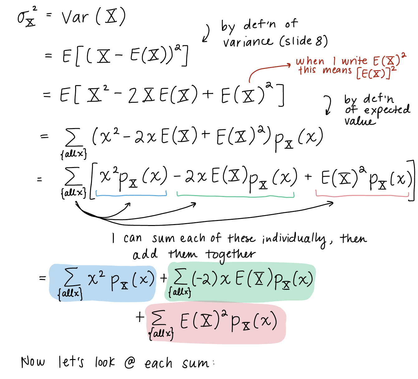
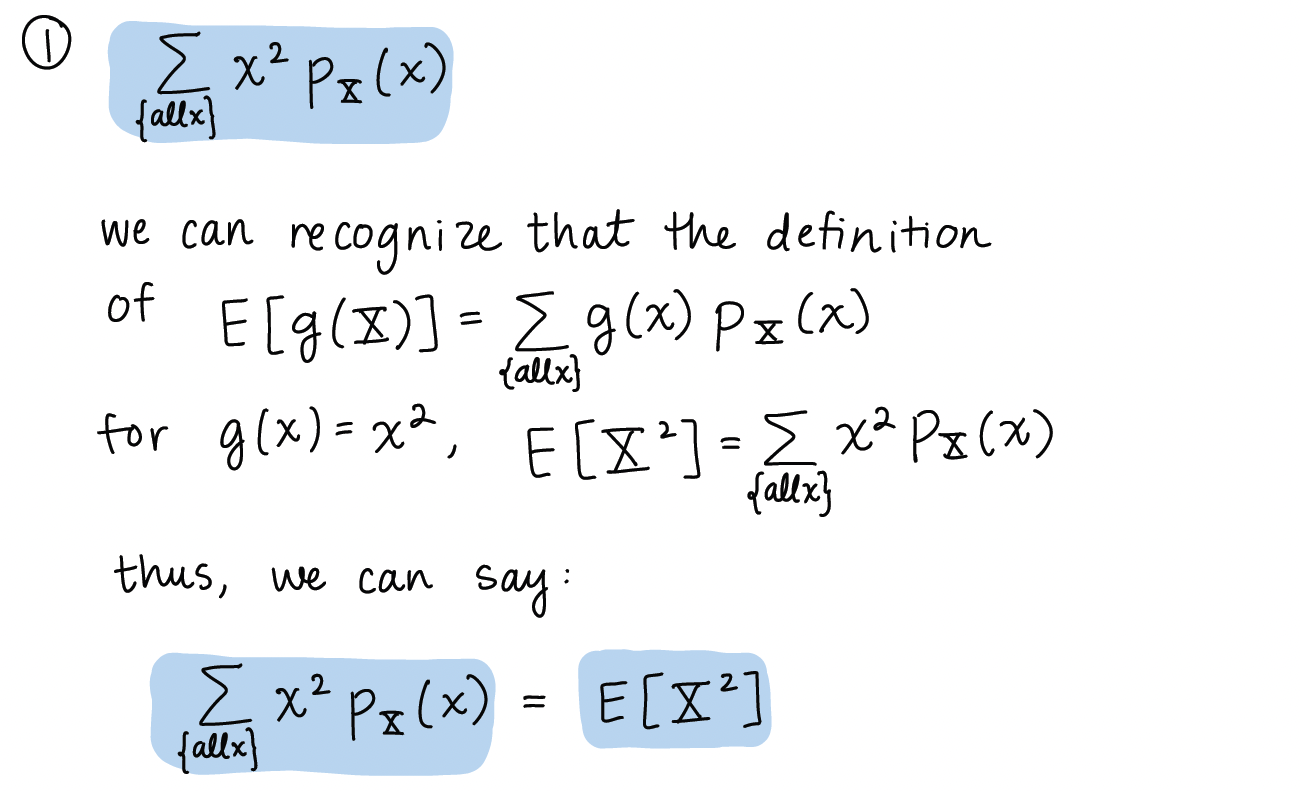
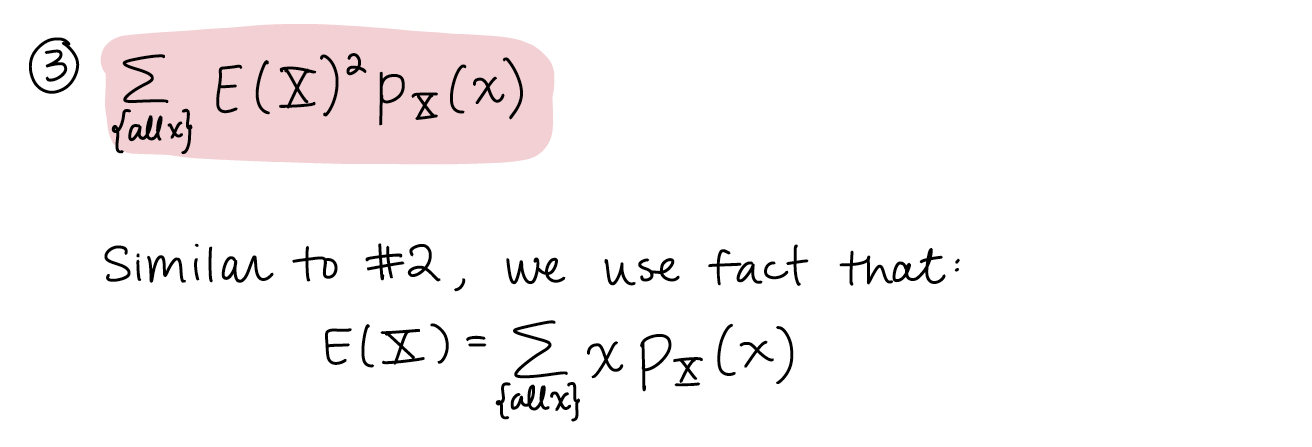
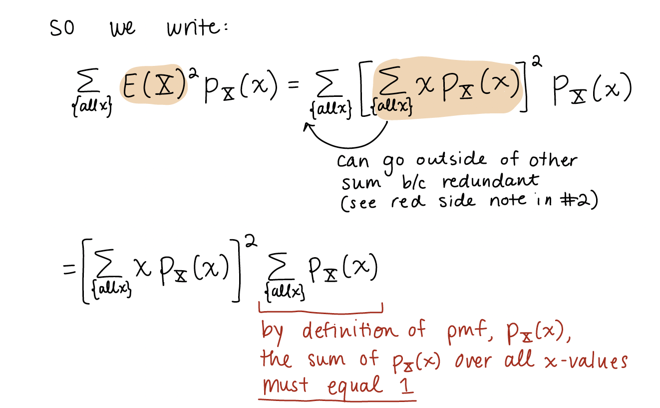
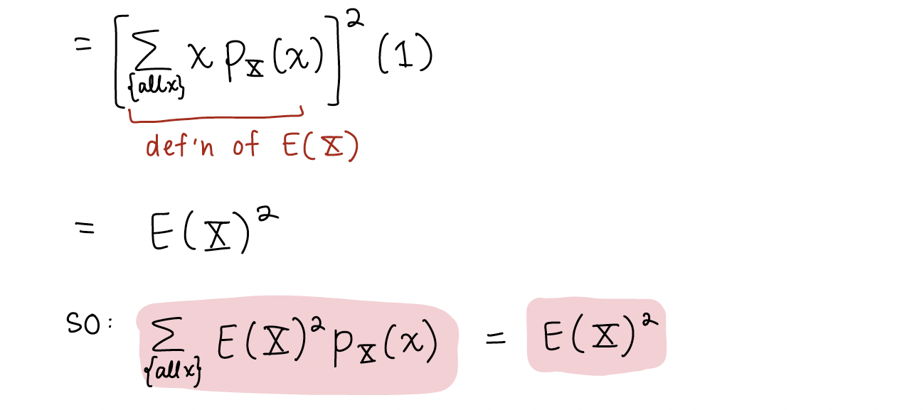
1. Proof of variance formula
Here is the variance formula that we worked through in class:
I stepped through this quite quickly and made some implicit steps. So let’s revisit it with explicit steps!
2. What progression are we following in the course??
Someone asked if this is our progression: RV is function \(\to\) Expected value is function to describe mean of RV \(\to\) Use functions within expected value to set up variance
Basically, yes! The random variable is a function of a random process. The RV inherits that randomness.
From there, we’ve been working towards calculating the probability of a realized value (\(x\)) of the RV. The probability can be different for different realized values (as it links back to the random process).
We also want to construct ways to describe our random variables. We may want to figure out what to expect from our random variable (which translates to the mean value of the RV). Since our RV is rooted in a random process, we may want to get an idea of how spread out our realized values are. We use our expected value (mean) as an anchor in our spread. Variance is one way to measure this spread.