Lesson 16: Some Important Continuous RVs

Meike Niederhausen and Nicky Wakim

2025-11-19

Learning Objectives

Distinguish between Uniform, Exponential, Gamma, and Normal distributions when reading a word problem.
Identify the variable and the parameters in a word problem, and state what the variable and parameters mean.
Use the formulas for the pdf/CDF, expected value, and variance to answer questions and find probabilities.

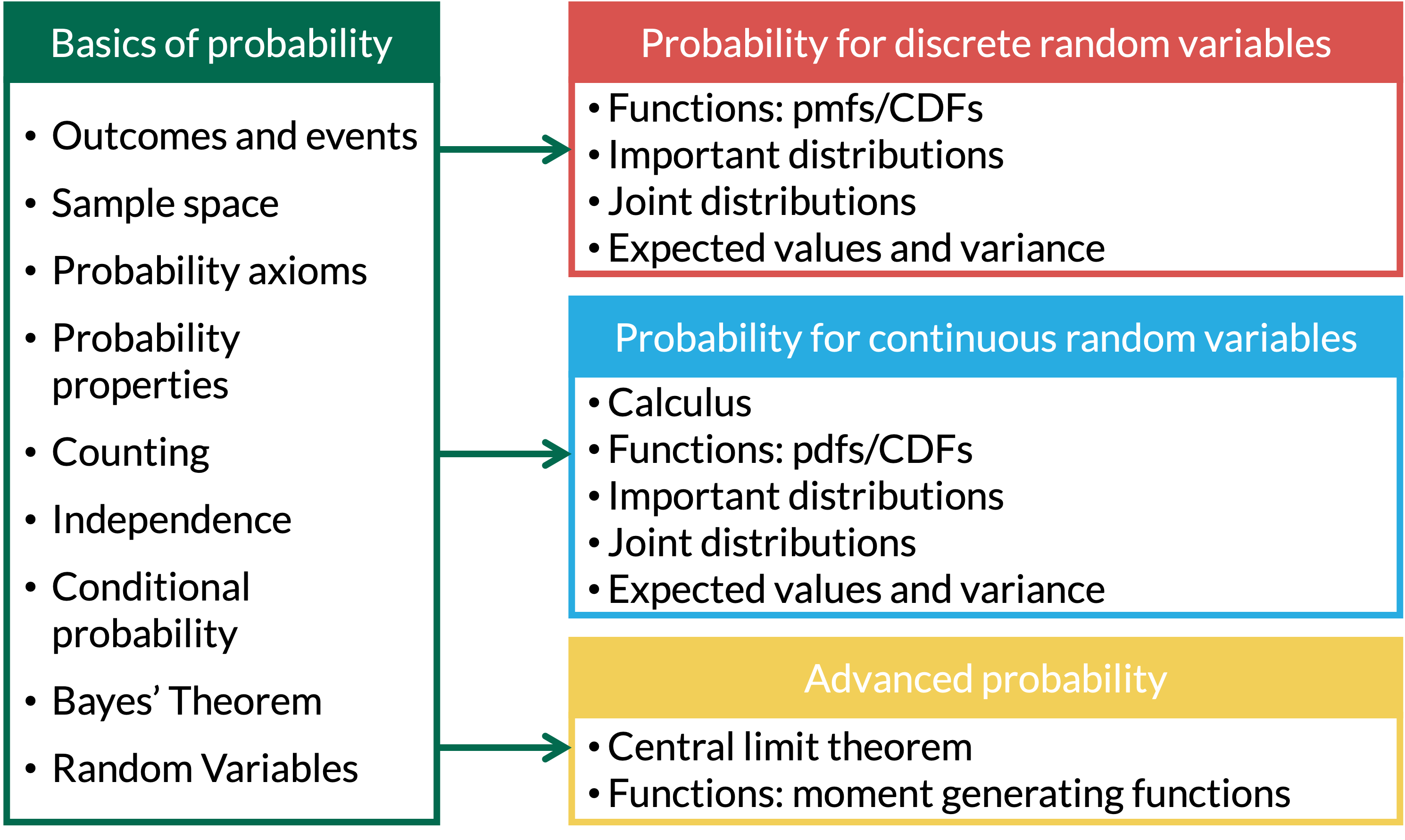
Where are we?

Continuous uniform RVs

Properties of continuous uniform RVs

Scenario: Events are equally likely to happen anywhere or anytime in an interval of values
Shorthand: \(X \sim \text{U}[a,b]\)

\[ f_X(x) = \dfrac{1}{b-a}, \text{ for }a \leq x \leq b \]

\[ F_X(x) = \left\{ \begin{array}{ll} 0 & \quad x<a \quad \\ \dfrac{x-a}{b-a} & \quad a \leq x \leq b\quad \\ 1 & \quad x>b \quad \end{array} \right. \]

\[\text{E}(X) = \dfrac{a+b}{2} \text{, } \text{ Var}(X) = \dfrac{(b-a)^2}{12}\]

Identifying continuous uniform RV from word problems

Look for some indication that all events are equally likely
- Could also say “uniformly distributed”
Look for an interval
- Time example: Costumer in your store will approach the cash register in next 30 minutes. Approaching the register throughout the 30 minutes is equally likely.
- Length example: You have a 12 inch string that you need to cut. You are equally likely to cut anywhere on the string.
Different than the discrete uniform
- Discrete usually includes a countable number of events that are equally likely
- Continuous is not countable
  - Exact time and length can be measured with infinite decimal places

Helpful R code

Let’s say we’re looking at equally likely arrival times between 10 am and 11 am.

If we want to know the probability that someone arrives at 10:30am or earlier:
```
punif(q = 30, min = 0, max = 60)
```
```
[1] 0.5
```
If we want to know the time, say \(t\), where the probability of arriving at \(t\) or earlier is 0.35:
```
qunif(p = 0.35, min = 0, max = 60)
```
```
[1] 21
```

If we want to know the probability that someone arrives between 10:14 and 10:16 am:

punif(q = 16, min = 0, max = 60) - punif(q = 14, min = 0, max = 60)

[1] 0.03333333

If we want to sample 20 arrival times from the distribution:

runif(n = 20, min = 0, max = 60)

 [1] 57.254766 34.877635  9.463305  9.299211 44.853180 24.713062  7.637811
 [8] 56.432479 57.911681 26.541762 41.756752 32.239442 54.968374  4.029851
[15] 33.138835 40.718886  5.610676 19.739926 21.084020 36.677654

Bird on a wire (TB 31.5)

Example 1

A bird lands at a location that is Uniformly distributed along an electrical wire of length 150 feet. The wire is stretched tightly between two poles. What is the probability that the bird is 20 feet or less from one or the other of the poles?

Exponential RVs

Properties of exponential RVs

Scenario: Modeling the time until the next (first) event
Continuous analog to the geometric distribution!
Shorthand: \(X \sim \text{Exp}(\lambda)\)

\[ f_X(x) = \lambda e^{-\lambda x}\text{ for } x>0, \lambda>0 \]

\[ F_X(x) = \left\{ \begin{array}{ll} 0 & \quad x<0 \quad \\ 1 - e^{-\lambda x} & \quad x\geq0 \\ \end{array} \right. \]

\[\text{E}(X) = \dfrac{1}{\lambda}\] \[\text{Var}(X) = \dfrac{1}{\lambda^2}\]

Memoryless Property

If \(b>0\),

\[P(X > a +b | X> a) = P(X > b)\]

This can be interpreted as:
- If you have waited \(a\) seconds (or any other measure of time) without a success
- Then the probability that you have to wait \(b\) more seconds is the same as as the probability of waiting \(b\) seconds initially.

Identifying exponential RV from word problems

Look for time between events/successes
Look for a rate of the events over time period
How does it differ from the geometric distribution?
- Geometric is number of trials until first success
- Exponential is time until first success
Relation to the Poisson distribution?
- When the time between arrivals is exponential, the number of arrivals in a fixed time interval is Poisson with the mean \(\lambda\)

Helpful R code

Let’s say we’re sitting at the bus stop, measuring the time until our bus arrives. We know the bus comes every 10 minutes on average.

If we want to know the probability that the bus arrives in the next 5 minutes:
```
pexp(q = 5, rate = 1/10)
```
```
[1] 0.3934693
```
If we want to know the time, say \(t\), where the probability of the bus arriving at \(t\) or earlier is 0.35:
```
qexp(p = 0.35, rate = 1/10)
```
```
[1] 4.307829
```
If we want to know the probability that the bus arrives between 3 and 5 minutes:
```
pexp(q = 5, rate = 1/10) - pexp(q = 3, rate = 1/10)
```
```
[1] 0.1342876
```

If we want to sample 20 bus arrival times from the distribution:

rexp(n = 20, rate = 1/10)

 [1]  3.27079121  9.21887422 23.15584516  1.43197788  7.13709980  2.46155182
 [7]  1.25854357 16.49368095  2.07284506  9.61934986  1.72675516  9.66994375
[13]  0.60112111  8.14090359 27.93188929  0.02541741 22.76283795  4.51165567
[19] 15.79182468  2.31727717

Transformation of independent exponential RVs

Revisit after joint notes:

Example 2

Let \(X_i \sim \textrm{Exp}(\lambda_i)\) be independent RVs, for \(i=1 \ldots n\). Find the pdf for the first of the arrival times.

Gamma RVs

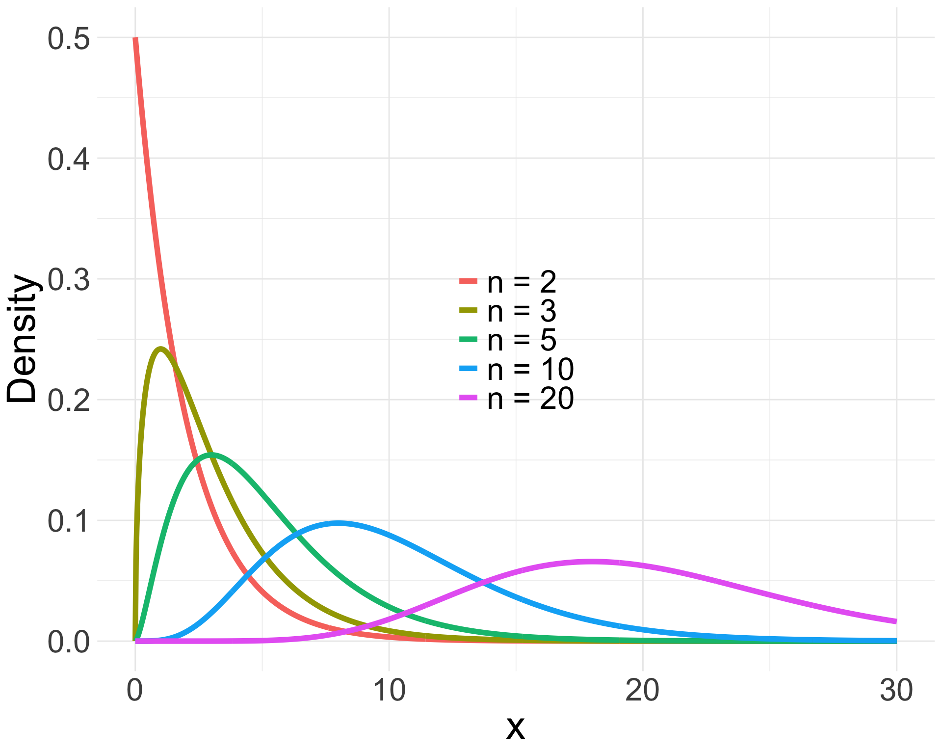
Properties of gamma RVs

Scenario: Modeling the time until the \(r^{th}\) event.
Continuous analog to the Negative Binomial distribution
Shorthand: \(X \sim \text{Gamma}(r, \lambda)\) or \(X \sim \text{Gamma}(\alpha, \beta)\)

\[ f_X(x) = \dfrac{\lambda^r}{\Gamma(r)}x^{r-1} e^{-\lambda x}\text{ for } x>0, \lambda>0, \Gamma(r) = (r-1)! \]

\[ F_X(x) = \left\{ \begin{array}{ll} 0 & \quad x<0 \quad \\ 1 - e^{-\lambda x}\displaystyle\sum_{j=0}^{r-1}\dfrac{(\lambda x)^j}{j!} & \quad x\geq0 \\ \end{array} \right. \]

\[\text{E}(X) = \dfrac{r}{\lambda}\text{, }\text{ Var}(X) = \dfrac{r}{\lambda^2}\]

Common to see \(\alpha = r\) and \(\beta = \lambda\)

Identifying gamma RV from word problems

Gamma distribution with \(r=1\) is same as exponential
- Just like Negative Binomial with \(r=1\) is same as the geometric distribution
Similar to exponential
- Look for time between or until events/successes
  - BUT now we are measuring time until more than 1 success
- Look for a rate of the events over time period

Helpful R code

Let’s say we’re sitting at the bus stop, measuring the time until 4 buses arrive. We know the bus comes every 10 minutes on average.

If we want to know the probability that the 4 buses arrive in the next 50 minutes:

pgamma(q = 50, rate = 1/10, shape = 4)

[1] 0.7349741

pgamma(q = 50, scale = 10, shape = 4)

[1] 0.7349741

If we want to know the time, say \(t\), where the probability of the 4 buses arriving at \(t\) or earlier is 0.35:
```
qgamma(p = 0.35, rate = 1/10, shape = 4)
```
```
[1] 29.87645
```

If we want to know the probability that the 4 buses arrives between 30 and 50 minutes:

pgamma(q = 50, scale = 10, shape = 4) - pgamma(q = 30, scale = 10, shape = 4)

[1] 0.382206

If we want to sample 20 arrival times for the 4 buses:

rgamma(n = 20, scale = 10, shape = 4)

 [1] 67.04894 14.44306 43.05435 12.51608 30.58018 34.94098 28.34891 26.01258
 [9] 37.60928 24.73837 32.30761 45.71904 54.58035 41.08169 18.69450 28.78482
[17] 51.66387 40.08829 56.18500 22.85659

Remarks

The parameter \(r\) in a Gamma(\(r\),\(\lambda\)) distribution does NOT need to be a positive integer
- \(r\) is usually a positive integer
When \(r\) is a positive integer, the distribution is sometimes called an Erlang(\(r\),\(\lambda\)) distribution
When \(r\) is any positive real number, we have a general gamma distribution that is usually instead parameterized by \(\alpha>0\) and \(\beta>0\), where:
- \(\alpha = \text{shape parameter}\) : same as \(k\), the total number of events we must witness
  - In R code example: 4 buses to wait for
- \(\beta = \text{scale parameter}\) : same as \(\lambda\), the rate parameter
  - In R code example: 1 bus per 10 minutes (1/10)

Sending money orders

Example 3

On average, someone sends a money order once per 15 minutes. What is the probability someone sends 10 money orders in less than 3 hours?

Additional Resource

Another helpful site with R code: https://rpubs.com/mpfoley73/459051

Normal RVs

Properties of Normal RVs

No scenario description here because the Normal distribution is so universal
- Central Limit Theorem (next class) makes it applicable to many types of events
Shorthand: \(X \sim \text{Normal}(\mu, \sigma^2)\)

\[ f_X(x) = \dfrac{1}{\sqrt{2\pi \sigma^2}}e^{-(x-\mu)^2/(2\sigma^2)} \text{, for} -\infty < x < \infty \]

\[\text{E}(X) = \mu \] \[\text{Var}(X) = \sigma^2\]

Helpful R code

Let’s say we’re measuring the high temperature today. The average high temperature on this day across many, many years is 50 degrees with a standard deviation of 4 degrees.

If we want to know the probability that the high temperature is below 45 degrees:
```
pnorm(q = 45, mean = 50, sd = 4)
```
```
[1] 0.1056498
```
If we want to know the temoerature, say \(t\), where the probability of that the temperature is at \(t\) or lower is 0.35:
```
qnorm(p = 0.35, mean = 50, sd = 4)
```
```
[1] 48.45872
```

If we want to know the probability that the temperature is between 45 and 50 degrees:

pnorm(q = 50, mean = 50, sd = 4) - pnorm(q = 45, mean = 50, sd = 4)

[1] 0.3943502

If we want to sample 20 days’ temperature (over the years) from the distribution:

rnorm(n = 20, mean = 50, sd = 4)

 [1] 51.25746 45.35334 49.66657 51.78714 47.45682 53.39772 52.86730 47.12661
 [9] 49.79689 52.23243 50.95174 58.17850 51.36292 46.18399 52.27518 53.80362
[17] 51.33378 49.25484 54.50188 55.77698

Movie night while studying

Example 4

Children’s movies run an average of 98 minutes with a standard deviation of 10 minutes. You check out a random movie from the library to entertain your kids so you can study for your test. Assume that your kids will be occupied for the entire length of the movie.

What is the probability that your kids will be occupied for at least the 2 hours you would like to study?
What is range for the bottom quartile (lowest 25%) of time they will be occupied?

Standard Normal Distribution

\[ Z \sim \text{Normal}(\mu = 0, \sigma^2 = 1)\]

Used to be more helpful when computing was not as advanced
- Use tables of the standard normal
- You can convert any normal distribution to a standard normal through transformation
\(Z = \dfrac{X - \mu_X}{\sigma_X}\)
- Comes from \(X = \sigma_X Z + \mu_X\)
- Since \(\sigma_X\) and \(\mu_X\) are constants, then \(E(X) = \mu_X\) and \(SD(X) = \sigma_X\)

Chi-squared distribution

If \(Z \sim \text{Normal}(0,1)\), then \(X = Z^2\) has a Chi-squared distribution with 1 degree of freedom
- Shorthand: \(X \sim \chi^2_{(1)}\)
If \(Z_1, Z_2, \ldots, Z_n\) are independent standard normal RVs, then

\[X = \sum_{i=1}^n Z_i^2\]

has a Chi-squared distribution with \(n\) degrees of freedom
- Shorthand: \(X \sim \chi^2_{(n)}\)