Lesson 3: Language of Probability

Nicky Wakim

2026-10-05

Learning Objectives

Use set notation, Venn diagrams, and the concepts of unions, intersections, complements, and mutually exclusive events to represent and describe events.
Apply the axioms of probability and related properties to calculate probabilities and prove simple results.
Explain and use De Morgan’s Laws to simplify and solve probability problems.
Connect partitions and all rules of probability to calculate probabilities.

Where are we?

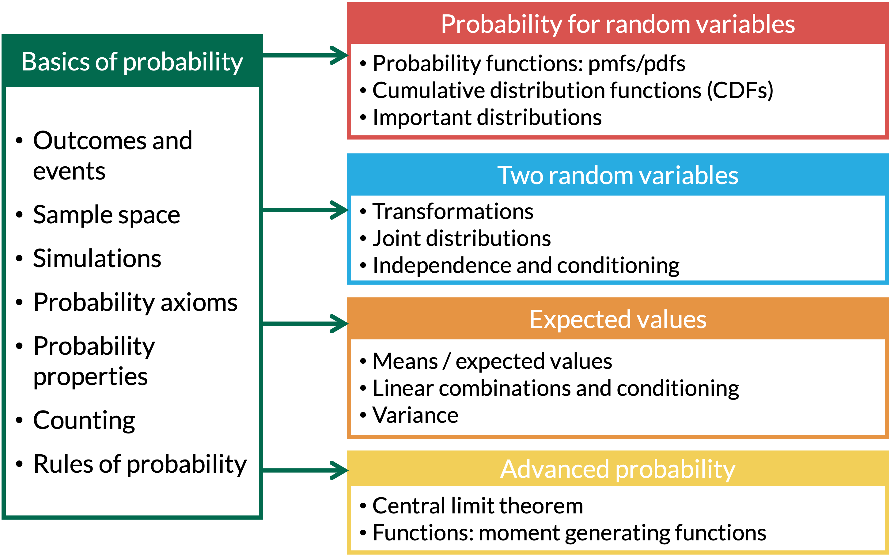
Learning Objectives

Use set notation, Venn diagrams, and the concepts of unions, intersections, complements, and mutually exclusive events to represent and describe events.

Apply the axioms of probability and related properties to calculate probabilities and prove simple results.
Explain and use De Morgan’s Laws to simplify and solve probability problems.
Connect partitions and all rules of probability to calculate probabilities.

Set Theory (1/2)

Definition: Union

The union of events $A$ and $B$, denoted by $A \cup B$, contains all outcomes that are in $A$ or $B$ or both

Definition: Intersection

The intersection of events $A$ and $B$, denoted by $A \cap B$, contains all outcomes that are both in $A$ and $B$.

Set Theory (2/2)

Definition: Complement

The complement of event $A$, denoted by $A^C$ or $A'$, contains all outcomes in the sample space $S$ that are not in $A$ .

Definition: Mutually Exclusive

Events $A$ and $B$ are mutually exclusive, or disjoint, if they have no outcomes in common. In this case $A \cap B = \emptyset$, where $\emptyset$ is the empty set.

How can we code some of these? (1/4)

Example 1: Simulating Two Rolls of a Fair Four-Sided Die

We’re going to roll two four-sided dice. This time, let’s say event A is rolling matching numbers, event B is rolling at least one 2, and event C is the sum of the dice is 5

First, we simulate rolling two four-sided dice. We start small, with only 5 simulations, so we can see every roll

set.seed(1022)
reps <- 5
n_dice <- 2
rolls <- expand_grid(sim = 1:reps, die = 1:n_dice) |>
  mutate(roll = sample(1:4, n(), replace = TRUE))

1: Set the seed once, so we get the same “random” rolls every time the slides are made.
2: Save the number of simulations and the number of dice as named values, so they are easy to change later.
3: Same setup as Lesson 2: one row for every combination of simulation and die. The pipe |> passes the table to the next line.
4: mutate() adds a column called roll. n() is the number of rows, so every row gets one random roll from 1 to 4.

rolls

1: Typing a name prints it. Each simulation (sim) has two rows, one for each die.

# A tibble: 10 × 3
     sim   die  roll
   <int> <int> <int>
 1     1     1     4
 2     1     2     3
 3     2     1     2
 4     2     2     1
 5     3     1     1
 6     3     2     4
 7     4     1     2
 8     4     2     2
 9     5     1     3
10     5     2     3

How can we code some of these? (2/4)

Example 1: Simulating Two Rolls of a Fair Four-Sided Die

We’re going to roll two four-sided dice. This time, let’s say event A is rolling matching numbers, event B is rolling at least one 2, and event C is the sum of the dice is 5

Now, we make one row per simulation, with a TRUE/FALSE column for each event

event_sims <- rolls |>
  group_by(sim) |>
  summarise(A = n_distinct(roll) == 1,
            B = any(roll == 2),
            C = sum(roll) == 5)

1: Start with rolls and save the result as event_sims.
2: Group the rows by simulation, so the next line works on the two dice of each simulation together.
3: n_distinct() counts the different values. The dice match exactly when there is only 1 distinct value, so A is TRUE for matching rolls.
4: roll == 2 checks each die. any() is TRUE if at least one of them is a 2.
5: sum() adds the two dice, and == 5 checks if the total is 5.

event_sims

1: One row per simulation. TRUE means the event happened in that simulation.

# A tibble: 5 × 4
    sim A     B     C    
  <int> <lgl> <lgl> <lgl>
1     1 FALSE FALSE FALSE
2     2 FALSE TRUE  FALSE
3     3 FALSE FALSE TRUE 
4     4 TRUE  TRUE  FALSE
5     5 TRUE  FALSE FALSE

How can we code some of these? (3/4)

Union

$A \cup B$
A | B

event_sims$A | event_sims$B

1: $ pulls one column out of a table. | means “or”: the result is TRUE when A happens, B happens, or both.

[1] FALSE  TRUE FALSE  TRUE  TRUE

Complement

$A^c$ or $A'$
!A

!event_sims$A

1: ! means “not”: it flips every TRUE to FALSE and every FALSE to TRUE.

[1]  TRUE  TRUE  TRUE FALSE FALSE

Intersection

$A \cap B$
A & B

event_sims$A & event_sims$B

1: & means “and”: the result is TRUE only when A and B both happen.

[1] FALSE FALSE FALSE  TRUE FALSE

Mutually Exclusive

$A \cap C = \emptyset$
any(A & C) is FALSE

any(event_sims$A & event_sims$C)

1: A & C is TRUE when the dice match and sum to 5. any() checks if that ever happens. Matching dice always have an even sum, so it never does: A and C are mutually exclusive.

[1] FALSE

How can we code some of these? (4/4)

Example 1: Simulating Two Rolls of a Fair Four-Sided Die

We’re going to roll two four-sided dice. This time, let’s say event A is rolling matching numbers, event B is rolling at least one 2, and event C is the sum of the dice is 5

Same code, now with 10,000 simulations

reps <- 10000
rolls <- expand_grid(sim = 1:reps, die = 1:n_dice) |>
  mutate(roll = sample(1:4, n(), replace = TRUE))
event_sims <- rolls |>
  group_by(sim) |>
  summarise(A = n_distinct(roll) == 1,
            B = any(roll == 2),
            C = sum(roll) == 5)

1: The only change: 10,000 simulations instead of 5.
2: The rest is the same code as before.

Estimate the probabilities

event_sims |>
  summarise(p_A = mean(A),
            p_B = mean(B),
            p_A_and_B = mean(A & B),
            p_A_or_B = mean(A | B))

1: mean() of a TRUE/FALSE column is a proportion: TRUE counts as 1 and FALSE as 0. So mean(A) is the proportion of simulations where A happened.
2: We can use & and | right inside mean().

# A tibble: 1 × 4
    p_A   p_B p_A_and_B p_A_or_B
  <dbl> <dbl>     <dbl>    <dbl>
1 0.255 0.437    0.0676    0.624

Exact: $\frac{4}{16} = 0.25$, $\frac{7}{16} = 0.4375$, $\frac{1}{16} = 0.0625$, $\frac{10}{16} = 0.625$

Learning Objectives

Use set notation, Venn diagrams, and the concepts of unions, intersections, complements, and mutually exclusive events to represent and describe events.

Apply the axioms of probability and related properties to calculate probabilities and prove simple results.

Explain and use De Morgan’s Laws to simplify and solve probability problems.
Connect partitions and all rules of probability to calculate probabilities.

Probability Axioms

Axiom 1

For every event $A$, $0\leq\mathbb{P}(A)\leq 1$. Probability is between 0 and 1.

Axiom 2

For the sample space $S$, $\mathbb{P}(S)=1$.

Axiom 3

If $A_1, A_2, A_3, \ldots$, is a collection of disjoint events, then \[\mathbb{P}\Big( \bigcup \limits_{i=1}^{\infty}A_i\Big) = \sum_{i=1}^{\infty}\mathbb{P}(A_i).\] The probability of at least one $A_i$ is the sum of the individual probabilities of each.

Some probability properties

Using the Axioms, we can prove all other probability properties! Events A, B, and C are not necessarily disjoint!

Proposition 1

For any event $A$, $\mathbb{P}(A)= 1 - \mathbb{P}(A^C)$

Proposition 2

$\mathbb{P}(\emptyset)=0$

Proposition 3

If $A \subseteq B$, then $\mathbb{P}(A) \leq \mathbb{P}(B)$

Proposition 4

\[\mathbb{P}(A \cup B) = \mathbb{P}(A) + \mathbb{P}(B) - \mathbb{P}(A \cap B)\] where $A$ and $B$ are not necessarily disjoint

Proposition 5

$\begin{aligned} \mathbb{P}(A \cup B & \cup C) = \mathbb{P}(A) + \mathbb{P}(B) + \\ & \mathbb{P}(C) - \mathbb{P}(A \cap B) - \mathbb{P}(A \cap C) - \\ & \mathbb{P}(B \cap C) + \mathbb{P}(A \cap B \cap C) \end{aligned}$

Proposition 1 Proof

Proposition 1

For any event $A$, $\mathbb{P}(A)= 1 - \mathbb{P}(A^C)$

Use Axioms!

A1: $0\leq\mathbb{P}(A)\leq 1$

A2: $\mathbb{P}(S)=1$

A3: For disjoint $A_i$,

$\mathbb{P}\Big( \bigcup \limits_{i=1}^{\infty}A_i\Big) = \sum_{i=1}^{\infty}\mathbb{P}(A_i)$

Proposition 1 in our dice simulation

Proposition 1

For any event $A$, $\mathbb{P}(A)= 1 - \mathbb{P}(A^C)$

Two dice: B is “at least one 2”, so $B^C$ is “no 2s”

event_sims |>
  summarise(p_B = mean(B),
            p_B_comp = mean(!B),
            p_B_prop_1= 1 - mean(!B))

1: Back to our 10,000 simulations of two dice.
2: !B is the complement, $B^C$.
3: Proposition 1 says one minus its probability gives $\mathbb{P}(B)$.

# A tibble: 1 × 3
    p_B p_B_comp p_B_prop_1
  <dbl>    <dbl>      <dbl>
1 0.437    0.563      0.437

Exact: $1 - \mathbb{P}(B^C) = 1 - \left(\frac{3}{4}\right)^2 = \frac{7}{16} = 0.4375$

Proposition 2 Proof

Proposition 2

$\mathbb{P}(\emptyset)=0$

Use Axioms!

A1: $0\leq\mathbb{P}(A)\leq 1$

A2: $\mathbb{P}(S)=1$

A3: For disjoint $A_i$,

$\mathbb{P}\Big( \bigcup \limits_{i=1}^{\infty}A_i\Big) = \sum_{i=1}^{\infty}\mathbb{P}(A_i)$

Proposition 3 Proof

Proposition 3

If $A \subseteq B$, then $\mathbb{P}(A) \leq \mathbb{P}(B)$

Use Axioms!

A1: $0\leq\mathbb{P}(A)\leq 1$

A2: $\mathbb{P}(S)=1$

A3: For disjoint $A_i$,

$\mathbb{P}\Big( \bigcup \limits_{i=1}^{\infty}A_i\Big) = \sum_{i=1}^{\infty}\mathbb{P}(A_i)$

Proposition 4 Visual Proof

Proposition 4

$\mathbb{P}(A \cup B) = \mathbb{P}(A) + \mathbb{P}(B) - \mathbb{P}(A \cap B)$

Proposition 4 in our dice simulation

Proposition 4

$\mathbb{P}(A \cup B) = \mathbb{P}(A) + \mathbb{P}(B) - \mathbb{P}(A \cap B)$

A is matching numbers and B is at least one 2, so they overlap at (2, 2)

event_sims |>
  summarise(p_A_or_B = mean(A | B),
            add_subtract = mean(A) + mean(B) - mean(A & B))

1: Back to our 10,000 simulations of two dice.
2: The left side of Proposition 4: the proportion of simulations where A or B happened.
3: The right side: add the two proportions, then subtract the overlap once.

# A tibble: 1 × 2
  p_A_or_B add_subtract
     <dbl>        <dbl>
1    0.624        0.624

Exact: $\frac{4}{16} + \frac{7}{16} - \frac{1}{16} = \frac{10}{16} = 0.625$
The two columns match exactly, not just approximately

Proposition 5 Visual Proof

Proposition 5

$\mathbb{P}(A \cup B \cup C) = \mathbb{P}(A) + \mathbb{P}(B) + \mathbb{P}(C) - \mathbb{P}(A \cap B) - \mathbb{P}(A \cap C) - \mathbb{P}(B \cap C) + \mathbb{P}(A \cap B \cap C)$

Some final remarks on these propositions

Notice how we spliced events into multiple disjoint events
- It is often easier to work with disjoint events

If we want to calculate the probability for one event, we may need to get creative with how we manipulate other events and the sample space
- Helps us use any incomplete information we have

Learning Objectives

Use set notation, Venn diagrams, and the concepts of unions, intersections, complements, and mutually exclusive events to represent and describe events.
Apply the axioms of probability and related properties to calculate probabilities and prove simple results.

Explain and use De Morgan’s Laws to simplify and solve probability problems.

Connect partitions and all rules of probability to calculate probabilities.

De Morgan’s Laws

Theorem: De Morgan’s 1st Law

For a collection of events (sets) $A_1, A_2, A_3, \ldots$

\[\bigcap\limits_{i=1}^{n}A_i^C = \Big(\bigcup\limits_{i=1}^{n}A_i\Big)^C\]

“all not A = $($at least one event A$)^C$” or “intersection of the complements is the complement of the union”

Theorem: De Morgan’s 2nd Law

For a collection of events (sets) $A_1, A_2, A_3, \ldots$

\[\bigcup\limits_{i=1}^{n}A_i^C = \Big(\bigcap\limits_{i=1}^{n}A_i\Big)^C\]

“at least one event not A = $($all A$)^C$” or “union of complements is complement of the intersection”

Example 2: Blood Pressures (BPs)

Suppose you have $n$ subjects in a study. Let $H_i$ be the event that person $i$ has high BP, for $i=1\ldots n$.

Use set theory notation to denote the following events:

Event subject $i$ does not have high BP
Event all $n$ subjects have high BP
Event at least one subject has high BP
Event all of them do not have high BP
Event at least one subject does not have high BP

Example 2: Blood Pressures (BPs)

Suppose you have $n$ subjects in a study. Let $H_i$ be the event that person $i$ has high BP, for $i=1\ldots n$.

Use set theory notation to denote the following events:

Event subject $i$ does not have high BP

Event all $n$ subjects have high BP

Event at least one subject has high BP

Example 2: Blood Pressures (BPs)

Suppose you have $n$ subjects in a study. Let $H_i$ be the event that person $i$ has high BP, for $i=1\ldots n$.

Use set theory notation to denote the following events:

Event all of them do not have high BP

Event at least one subject does not have high BP

De Morgan’s Laws in simulation (1/2)

Simulate $n = 6$ subjects, each with a 30% chance of high BP, with 10,000 reps

n_subjects <- 6
p_high <- 0.3
subjects <- expand_grid(sim = 1:reps, subject = 1:n_subjects) |>
  mutate(status = sample(c("high", "normal"), n(), replace = TRUE,
                         prob = c(p_high, 1 - p_high)))
bp_sims <- subjects |>
  group_by(sim) |>
  summarise(all_not_high = all(status != "high"),    # Q2
            not_any_high = !any(status == "high"),   # Q3
            any_not_high = any(status != "high"),    # Q4
            not_all_high = !all(status == "high"))   # Q5
head(bp_sims, 3)

1: Save the number of subjects and the chance of high BP as named values, so they are easy to change.
2: Same pattern as the dice: one row for every combination of simulation and subject.
3: Like the unfair coin in Lesson 1: prob gives each label its own chance, here 30% “high” and 70% “normal”.
4: all() is TRUE only if every subject in the simulation meets the condition. This is $\bigcap H_i^C$, “all do not have high BP”.
5: !any() is “not (at least one has high BP)”, which is $\big(\bigcup H_i\big)^C$. De Morgan’s 1st Law says columns 4 and 5 are the same event.
6: The same for De Morgan’s 2nd Law: $\bigcup H_i^C$ (“at least one does not have high BP”) and $\big(\bigcap H_i\big)^C$ (“not all have high BP”).

# A tibble: 3 × 5
    sim all_not_high not_any_high any_not_high not_all_high
  <int> <lgl>        <lgl>        <lgl>        <lgl>       
1     1 FALSE        FALSE        TRUE         TRUE        
2     2 FALSE        FALSE        TRUE         TRUE        
3     3 FALSE        FALSE        TRUE         TRUE

De Morgan’s Laws in simulation (2/2)

Check that each pair of columns agrees in every simulation

bp_sims |>
  summarise(law_1_agree = mean(all_not_high == not_any_high),
            law_2_agree = mean(any_not_high == not_all_high),
            p_at_least_one_high = 1 - mean(all_not_high))

1: Start with the 10,000 simulations, one row each.
2: == compares the two columns row by row. A proportion of 1 means they agree in all 10,000 simulations.
3: “At least one has high BP” is a union, which is hard to count directly. De Morgan plus Proposition 1 turns it into 1 minus an intersection: “all do not have high BP”.

# A tibble: 1 × 3
  law_1_agree law_2_agree p_at_least_one_high
        <dbl>       <dbl>               <dbl>
1           1           1               0.876

Exact: $1 - (0.7)^6 \approx 0.8824$
We can find the probability of “all do not have high BP” more easily in the coming chapters

Remarks on De Morgan’s Laws

These laws also hold for infinite collections of events.
Draw Venn diagrams to convince yourself that these are true!
These laws are very useful when calculating probabilities.
- This is because calculating the probability of the intersection of events is often much easier than the union of events.
- This is not obvious right now, but we will see in the coming chapters why.

Learning Objectives

Use set notation, Venn diagrams, and the concepts of unions, intersections, complements, and mutually exclusive events to represent and describe events.
Apply the axioms of probability and related properties to calculate probabilities and prove simple results.
Explain and use De Morgan’s Laws to simplify and solve probability problems.

Connect partitions and all rules of probability to calculate probabilities.

Partitions

Definition: Partition

A set of events $\{A_i\}_{i=1}^{n}$ create a partition of $A$, if

the $A_i$’s are disjoint (mutually exclusive) and
$\bigcup \limits_{i=1}^n A_i = A$

Note

If $A \subset B$, then $\{A, B \cap A^C\}$ is a set of partitions of $B$.
If $S = \bigcup \limits_{i=1}^n A_i$, and the $A_i$’s are disjoint, then the $A_i$’s are a partition of the sample space.

Creating partitions is sometimes used to help calculate probabilities, since by Axiom 3 we can add the probabilities of disjoint events.

Example 3: Weekly medications

If a subject has an

80% chance of taking their medication this week,
70% chance of taking their medication next week, and
10% chance of not taking their medication either week,

then find the probability of them taking their medication exactly one of the two weeks.

Hint: Draw a Venn diagram labelling each of the parts to find the probability.

Checking Example 3 with simulation

After solving with the Venn diagram: simulate the four disjoint pieces (a partition of the sample space) and check the given facts

cells <- c("both", "this only", "next only", "neither")
med_sims <- expand_grid(sim = 1:reps) |>
  mutate(cell = sample(cells, n(), replace = TRUE,
                       prob = c(0.6, 0.2, 0.1, 0.1)))
med_sims |>
  summarise(p_this = mean(cell %in% c("both", "this only")),
            p_next = mean(cell %in% c("both", "next only")),
            p_neither = mean(cell == "neither"),
            p_exactly_one = mean(cell %in% c("this only", "next only")))

1: The four pieces of the Venn diagram. They are disjoint and together make up the whole sample space, so they form a partition.
2: One row per simulation. With only one thing to simulate per week pair, expand_grid() just needs sim.
3: Each simulation lands in exactly one piece, with the probabilities from our Venn diagram.
4: %in% checks if cell is any of the listed pieces. “Took it this week” is the union of two disjoint pieces, so by Axiom 3 its probability is their sum.
5: Our answer: “exactly one week” is the union of the two “only” pieces.

# A tibble: 1 × 4
  p_this p_next p_neither p_exactly_one
   <dbl>  <dbl>     <dbl>         <dbl>
1  0.797  0.696     0.105         0.297

The first three columns should be close to the 0.8, 0.7, and 0.1 we were given. If they are, our partition is right, and the last column checks our answer.