[1] 882.474Lesson 2: Intro to data & numerical summaries
TB sections 1.2, 1.4
2025-10-01
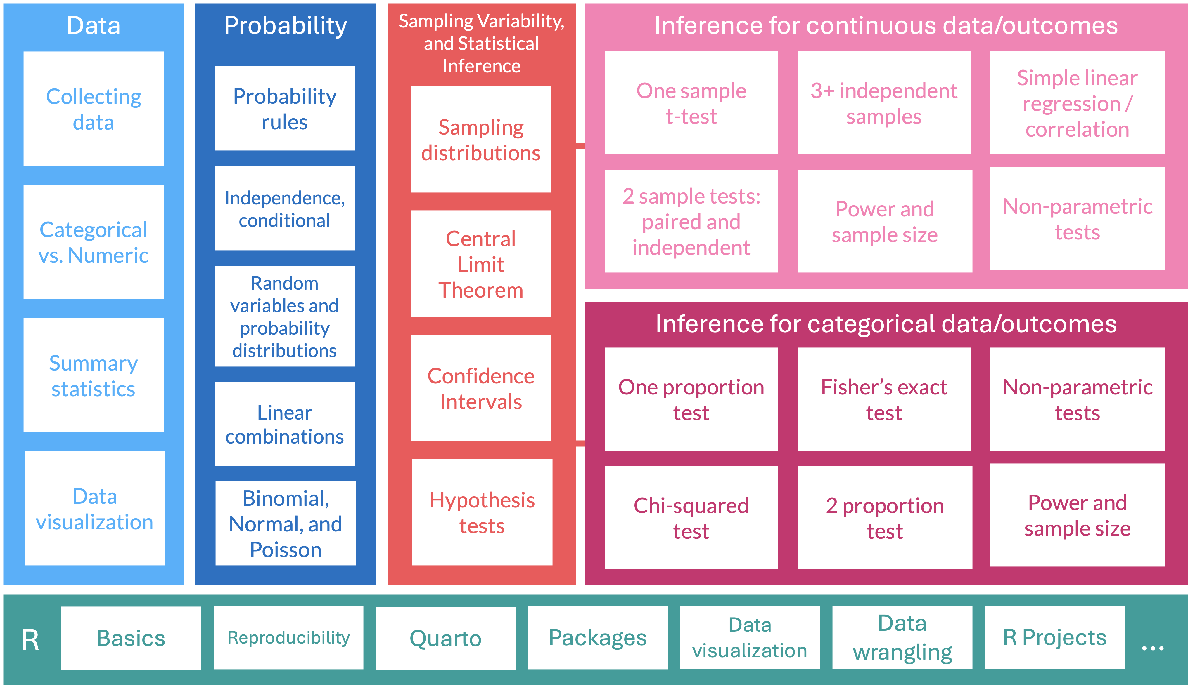
Where are we?
Intro to Data

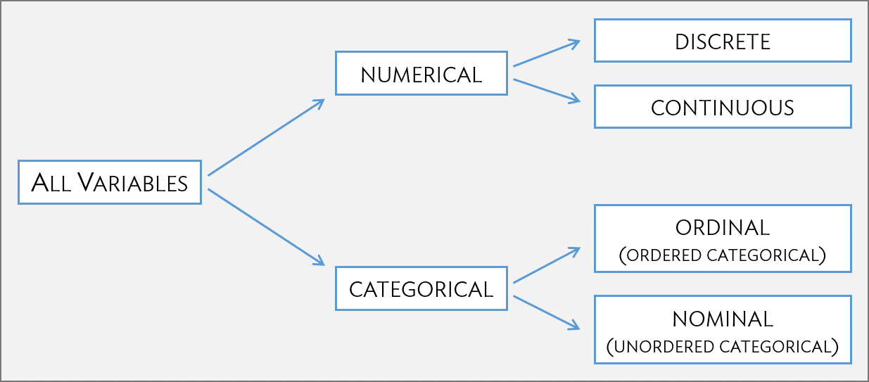
Types of variables (2/2)
Measures of center: mean vs. median
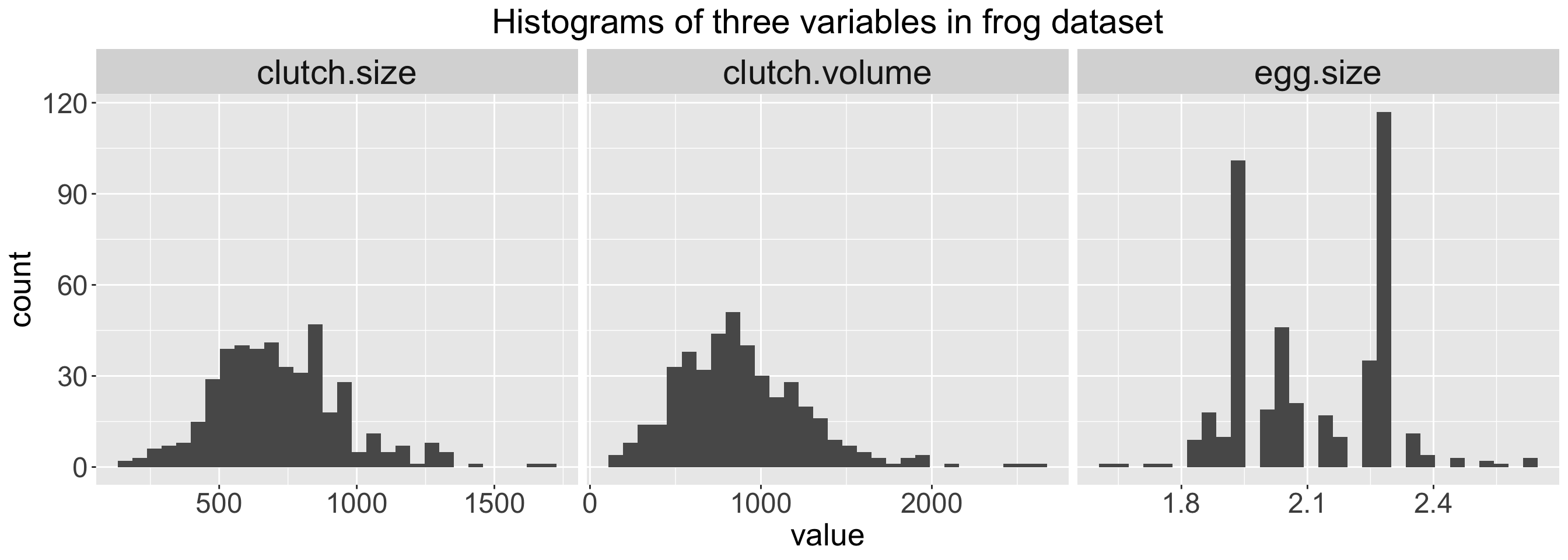
- Mean values will be pulled towards extreme values
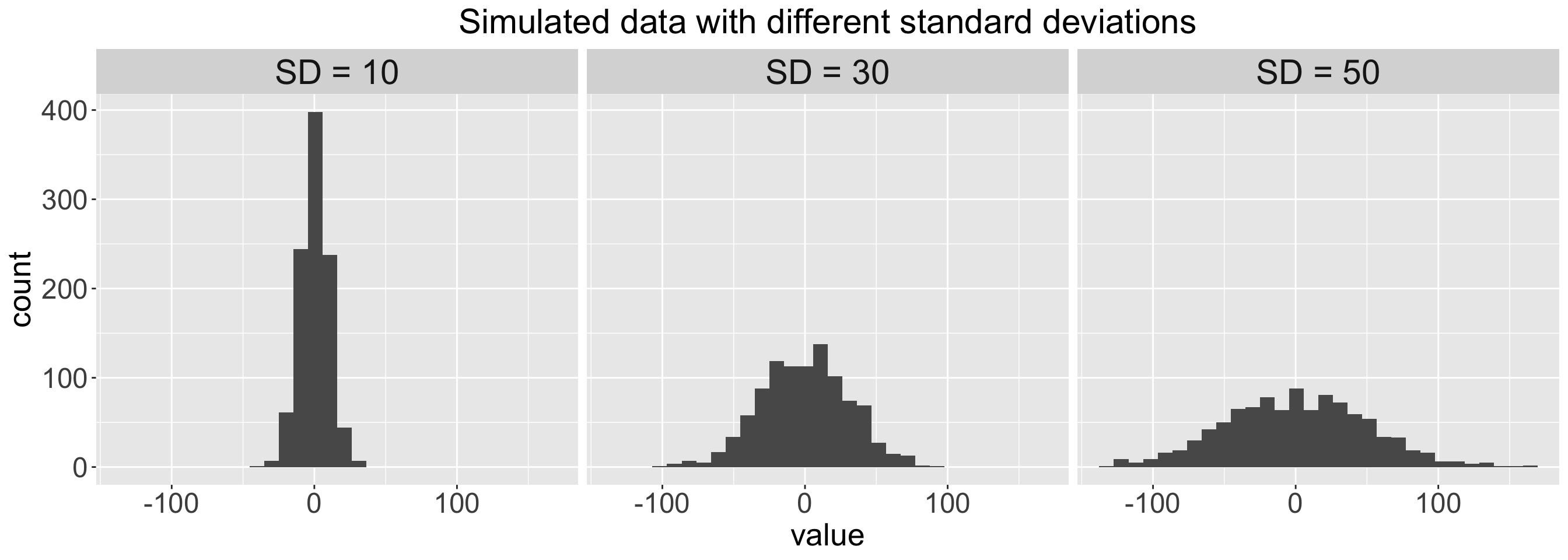
Measures of spread: standard deviation (SD) (1/3)
Standard deviation (SD)
(Approximately) the average distance between an observation and the mean
- An observation’s deviation is the distance between its value \(x\) and the sample mean \(\overline{x}\): deviation = \(x - \overline{x}\)
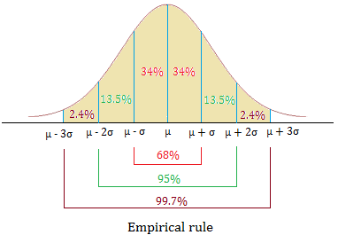
Empirical Rule: one way to think about the SD
For symmetric bell-shaped data, about
- 68% of the data are within 1 SD of the mean
- 95% of the data are within 2 SD’s of the mean
- 99.7% of the data are within 3 SD’s of the mean
These percentages are based off of percentages of a true normal distribution.
Measures of spread: IQR (2/2)
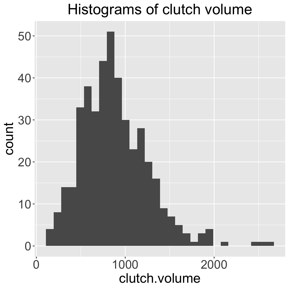
5 number summary
   Min. 1st Qu.  Median    Mean 3rd Qu.    Max.
  151.4   609.6   831.8   882.5  1096.5  2630.3
\[IQR = Q_3 - Q_1 = 1096.5 - 609.6 = 486.9\]