dbinom(x = 4, size = 10, prob = 0.25) # d for distribution[1] 0.145998TB sections 3.1-3.2
Random variable (RV or r.v.)
A random variable (r.v.) assigns numerical values (probability) to the outcome of a random phenomenon
Notation: A random variable is usually denoted with a capital letter such as \(X\), \(Y\), or \(Z\).
Probability distribution
A probability distribution consists of all disjoint outcomes and their associated probabilities.
Rules for a probability distribution
A probability distribution is a list of all possible outcomes and their associated probabilities that satisfies three rules:
We can start to define the probability distribution
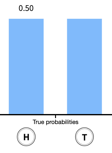
Let’s define the coin flip with the random variable \(X\)
We can create a table for the random variable and probabilities of each outcome:
| Coin flip (\(x\)) | \(x=1\) | \(x=0\) |
|---|---|---|
| Probability (\(P(X=x)\)) | 0.5 | 0.5 |
Example 1: Rolling a die
Suppose you roll a fair die. Let the random variable (r.v.) \(X\) be the outcome of the roll, i.e. the value of the face showing on the die.

Discrete random variable (RV)
A discrete RV \(X\) takes on a finite number of values or countably infinite number of possible values.
Think:
Continuous random variable (RV)
A continuous RV \(X\) can take on any real value in an interval of values or unions of intervals.
Think:
We call the mean of a random variable its expected value
The expected value is calculated as a weighted average
Expected value of a discrete random variable
If \(X\) takes on outcomes \(x_1\), …, \(x_k\) with probabilities \(P(X=x_1)\), …, \(P(X=x_k)\), the expected value of \(X\) is the sum of each outcome multiplied by its corresponding probability: \[\begin{aligned}\mu = E[X] = & x_1 P(X=x_1) + x_2 P(X=x_2) + \ldots + x_k P(X=x_k) \\ = & \sum_{i=1}^k x_iP(X=x_i) \end{aligned}\]
Example 1: Rolling a die
Let’s go back to our fair die with RV \(X\) as the value of the face showing on the die.
What is the expected outcome of the RV \(X\)?
Now suppose the 6-sided die is not fair. How would we calculate the expected outcome?
| \(x\) | \(\mathbb{P}(X=x)\) |
|---|---|
| 1 | 0.10 |
| 2 | 0.20 |
| 3 | 0.05 |
| 4 | 0.05 |
| 5 | 0.25 |
| 6 | 0.35 |
Just like with data, the variability of a r.v. is described with its variance or standard deviation
Variance of a discrete random variable
If \(X\) takes on outcomes \(x_1\), …, \(x_k\) with probabilities \(P(X=x_1)\), …, \(P(X=x_k)\) and expected value \(\mu=E(X)\), then the variance of \(X\), denoted by \(\text{Var}(X)\) or \(\sigma^2\), is
\[\begin{align*} \text{Var}(X) &= (x_1-\mu)^2 P(X=x_1) + \cdots+ (x_k-\mu)^2 P(X=x_k) \\ &= \sum_{i=1}^{k} (x_i - \mu)^2 P(X=x_i) \end{align*}\]
Standard deviation of a discrete random variable
The standard deviation of \(X\), labeled \(SD(X)\) or \(\sigma\), is \[\sigma = SD(X) = \sqrt{\text{Var}(X)} \]
Example 1: Rolling a die
Suppose you roll a fair 6-sided die. Let the random variable (r.v.)* \(X\) be the outcome of the roll, i.e. the value of the face showing on the die.
| \(x\) | \(\mathbb{P}(X=x)\) |
|---|---|
| 1 | 1/6 |
| 2 | 1/6 |
| 3 | 1/6 |
| 4 | 1/6 |
| 5 | 1/6 |
| 6 | 1/6 |
\[\begin{align*} \text{Var}(X) &= \sum_{i=1}^{6} (x_i - \mu)^2 P(X=x_i) \\ &= (1-3.5)^2 \frac{1}{6} + (2-3.5)^2 \frac{1}{6} + \\ \\ \\ \\ \\ \\ \\ \\ &= 2.917 \\ \\ \text{SD}(X) &= \end{align*}\]
Linear combinations of random variables
If \(X\) and \(Y\) are random variables and \(a\) and \(b\) are constants, then \[aX + bY\] is a linear combination of the random variables.
Theorem: Expected value of a linear combination of random variables
If \(X\) and \(Y\) are random variables and \(a\) and \(b\) are constants, then \[E(aX + bY) = aE(X) + bE(Y)\] and \[E(aX + b) = aE(X) + b\]
Example: Expected money for rolling 3 dice
Let the random variables \(X_1, X_2, X_3\) be the values shown on rolls for 2 fair 6-sided dice and 1 unfair die (as described in our previous example). Suppose you are given in dollars the amount of the first roll, plus twice the value of the second roll, plus 4 times the value of the unfair die roll. How much money do you expect to get?
Theorem: Variance of a linear combination of random variables
If \(X\) and \(Y\) are independent random variables and \(a\) and \(b\) are constants, then \[\text{Var}(aX +bY) = a^2\text{Var}(X) + b^2\text{Var}(Y)\]
Example: Expected money for rolling 3 dice
Let the random variables \(X_1, X_2, X_3\) be the values shown on rolls for 2 fair 6-sided dice and 1 unfair die (as described in our previous example). Suppose you are given in dollars the amount of the first roll, plus twice the value of the second roll, plus 4 times the value of the unfair die roll. What are the variance and standard deviation of the amount you get from the 3 rolls?
Binomial random variable
\(X\) is a binomial random variable if it represents the number of successes in \(n\) independent replications (or trials) of an experiment where
A binomial random variable takes on values \(0, 1, 2, \dots, n\).
If a r.v. \(X\) is modeled by a Binomial distribution, then we write in shorthand \(X \sim \text{Binom}(n,p)\)
Quick example: The number of heads in 3 tosses of a fair coin is a binomial random variable with parameters \(n = 3\) and \(p = 0.5\).
Bernoulli random variable
Bernoulli random variable. If \(X\) is a random variable that takes value 1 with probability of success \(p\) and 0 with probability \(1-p\) (or \(q\)), then \(X\) is a Bernoulli random variable.
We call the probability of success \(p\) the parameter of the Bernoulli distribution.
If a r.v. \(X\) is modeled by a Bernoulli distribution, then we write in shorthand \(X \sim \text{Bernoulli}(p)\) or \(X \sim \text{Bern}(p)\)
Mean and SD of a Bernoulli r.v.
If* \(X\) is a Bernoulli r.v. with probability of success \(p\), then \(E(X) = p\) and \(\text{Var}(X) = p(1-p)\)
The Bernoulli distribution is a special case of the Binomial distribution where \(n=1\)
To get a Binomial distribution, we simply extend the scenario from a single trial to multiple independent trials.
Quick example:
Distribution of a Binomial random variable
Let \(X\) be the total number of successes in \(n\) independent trials, each with probability \(p\) of a success. Then probability of observing exactly \(k\) successes in \(n\) independent trials is
\[P(X = x) = \binom{n}{x} p^x (1-p)^{n-x}, x= 0, 1, 2, \dots, n \]
The parameters of a binomial distribution are \(p\) and \(n\).
If a r.v. \(X\) is modeled by a binomial distribution, then we write in shorthand \(X \sim \text{Binom}(n,p)\)
Mean and variance of a Binomial r.v
If \(X\) is a binomial r.v. with probability of success \(p\), then \(E(X) = np\) and \(\text{Var}(X)=np(1-p)\)
R commands with their input and output:
| R code | What does it return? |
|---|---|
rbinom() |
returns sample of random variables with specified binomial distribution |
dbinom() |
returns probability of getting certain number of successes |
pbinom() |
returns cumulative probability of getting certain number or less successes |
qbinom() |
returns number of successes corresponding to desired quantile |
Vaccinated people testing positive for Covid-19
About 25% of people that test positive for Covid-19 are vaccinated for Covid-19. Suppose 10 people have tested positive for Covid-19 (independently of each other). Let \(X\) denote the number of people that are vaccinated among the 10 that tested positive.
What is the expected value of \(X\)?
What is the SD of \(X\)?
What is the probability that exactly 4 of the 10 people that tested positive are vaccinated?
What is the probability that at most 3 of the 10 people that tested positive are vaccinated?
What is the probability that at least 5 of the 10 people that tested positive are vaccinated?
Vaccinated people testing positive for Covid-19
About 25% of people that test positive for Covid-19 are vaccinated for Covid-19. Suppose 10 people have tested positive for Covid-19 (independently of each other). Let \(X\) denote the number of people that are vaccinated among the 10 that tested positive.
What is the expected value of \(X\)?
What is the SD of \(X\)?
Vaccinated people testing positive for Covid-19
About 25% of people that test positive for Covid-19 are vaccinated for Covid-19. Suppose 10 people have tested positive for Covid-19 (independently of each other). Let \(X\) denote the number of people that are vaccinated among the 10 that tested positive.
\[P(X=4) = {10 \choose 4} 0.25^2 (1-0.25)^{10-4} = 0.146\]
dbinom(x = 4, size = 10, prob = 0.25) # d for distribution[1] 0.145998dbinom(x = k, size = n, prob = p)Vaccinated people testing positive for Covid-19
About 25% of people that test positive for Covid-19 are vaccinated for Covid-19. Suppose 10 people have tested positive for Covid-19 (independently of each other). Let \(X\) denote the number of people that are vaccinated among the 10 that tested positive.
\[\begin{aligned} P(X \leq 3) = & P(X =0) + P(X = 1) + P(X =2) + P(X = 3) \\ = &{10 \choose 0} 0.25^0 (0.75)^{10} + {10 \choose 1} 0.25^1 (0.75)^{9} + {10 \choose 2} 0.25^2 (0.75)^{8}+ {10 \choose 3} 0.25^3 (0.75)^{7} \\ = & 0.7758 \end{aligned}\]
pbinom(q = 3, size = 10, prob = 0.25, lower.tail = T)[1] 0.7758751pbinom(q = k, size = n, prob = p) with lower.tail = T as a default optionVaccinated people testing positive for Covid-19
About 25% of people that test positive for Covid-19 are vaccinated for Covid-19. Suppose 10 people have tested positive for Covid-19 (independently of each other). Let \(X\) denote the number of people that are vaccinated among the 10 that tested positive.
\[\begin{aligned} P(X \geq 5) = & P(X =5) + P(X = 6) + P(X =7) + P(X = 8) + P(X = 9)+ P(X = 10) \\ = &{10 \choose 5} 0.25^5 (0.75)^{5} + {10 \choose 6} 0.25^6 (0.75)^{4} + \ldots + {10 \choose 10} 0.25^10 (0.75)^{0}\\ = & 0.7758 \end{aligned}\]
pbinom(q = 4, size = 10, prob = 0.25, lower.tail = F) # for greater than![1] 0.078126911 - pbinom(q = 4, size = 10, prob = 0.25, lower.tail = T)[1] 0.07812691pbinom(q = k, size = n, prob = p, lower.tail = F)Information on slide heavily borrowed from ChatGPT with prompt: “can you explain how we go from a bernoulli distribution to a binomial”↩︎