Lesson 6: Normal and Poisson distributions

TB sections 3.3-3.4

Meike Niederhausen and Nicky Wakim

2024-10-16

Learning Objectives

1. Understand how probability distributions extend to continuous distributions
2. Calculate probabilities for specific events using a Normal distribution
3. Apply the Normal distribution to approximate probabilities for binomial events
4. Calculate probabilities for different events using a Poisson distribution

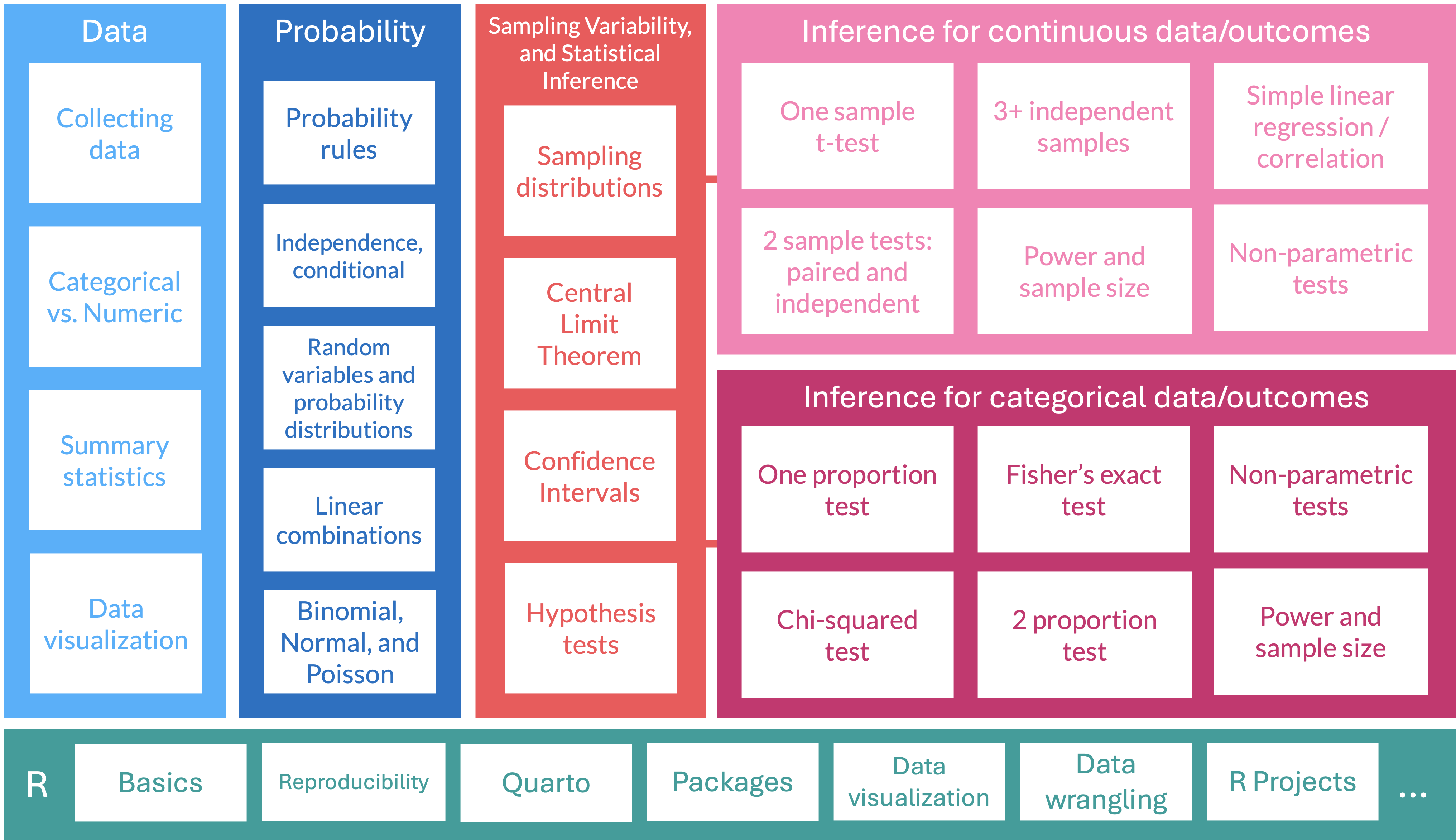
Where are we?

Learning Objectives

1. Understand how probability distributions extend to continuous distributions

2. Calculate probabilities for specific events using a Normal distribution
3. Apply the Normal distribution to approximate probabilities for binomial events
4. Calculate probabilities for different events using a Poisson distribution

Last time: Discrete vs. continuous random variables

• Probability distributions are usually either discrete or continuous, depending on whether the random variable is discrete or continuous.

Discrete random variable

A discrete r.v. \(X\) takes on a finite number of values or countably infinite number of possible values.

Think:

• Number of heads in a set of coin tosses
• Number of people who have had chicken pox in a random sample

 

• Binomial and Bernoulli distributions are discrete

Continuous random variable

A continuous r.v. \(X\) can take on any real value in an interval of values or unions of intervals.

Think:

• Height in a population
• Blood pressure in a population

Probabilities for continuous distributions (1/2)

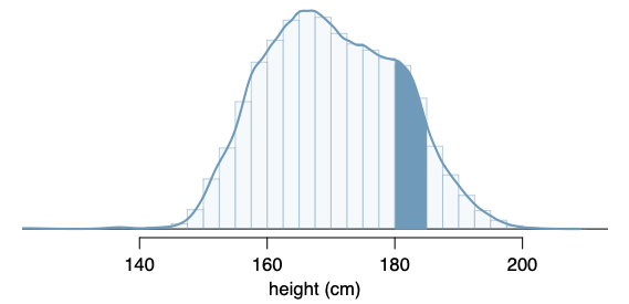
Two important features of continuous distributions:

• The total area under the density curve is 1.

• The probability that a variable has a value within a specified interval is the area under the curve over that interval.

Probabilities for continuous distributions (2/2)

When working with continuous random variables, probability is found for intervals of values rather than individual values.

• The probability that a continuous r.v. \(X\) takes on any single individual value is 0

  • That is, \(P(X = x) = 0\).

• Thus, \(P(a < X < b)\) is equivalent to \(P(a \leq X \leq b)\)

Poll Everywhere Question 1

Learning Objectives

1. Understand how probability distributions extend to continuous distributions

2. Calculate probabilities for specific events using a Normal distribution

3. Apply the Normal distribution to approximate probabilities for binomial events
4. Calculate probabilities for different events using a Poisson distribution

Normal distribution

• A random variable X is modeled with a normal distribution if:

  • Shape: symmetric, unimodal bell curve
  • Center: mean \(\mu\)
  • Spread (variability): standard deviation \(\sigma\)

 

• Shorthand for a random variable, \(X\), that has a Normal distribution: \[X \sim \text{Normal}(\mu, \sigma)\]

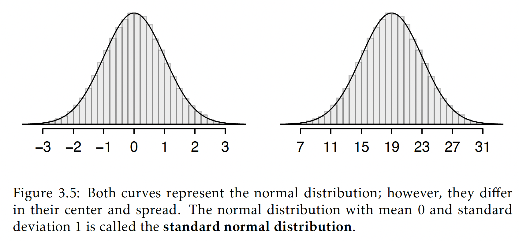
• Example: We recorded the high temperature in the past 100 years for today. The mean high is 19°C (66.2°F)

Standard Normal distribution (1/2)

• A standard normal distribution is defined as a normal distribution with mean 0 and variance 1. It is often denoted as \(Z \sim N(0, 1)\).

• Any normal random variable \(X\) can be transformed into a standard normal random variable \(Z\).

\[Z = \dfrac{X - \mu}{\sigma} \qquad X = \mu + Z\sigma\]

• The \(Z\)-score of an observation quantifies how far the observation is from the mean, in units of standard deviation(s).

• For example, if an observation has \(Z\)-score \(z = 3.4\), then the observation is 3.4 standard deviations above the mean.

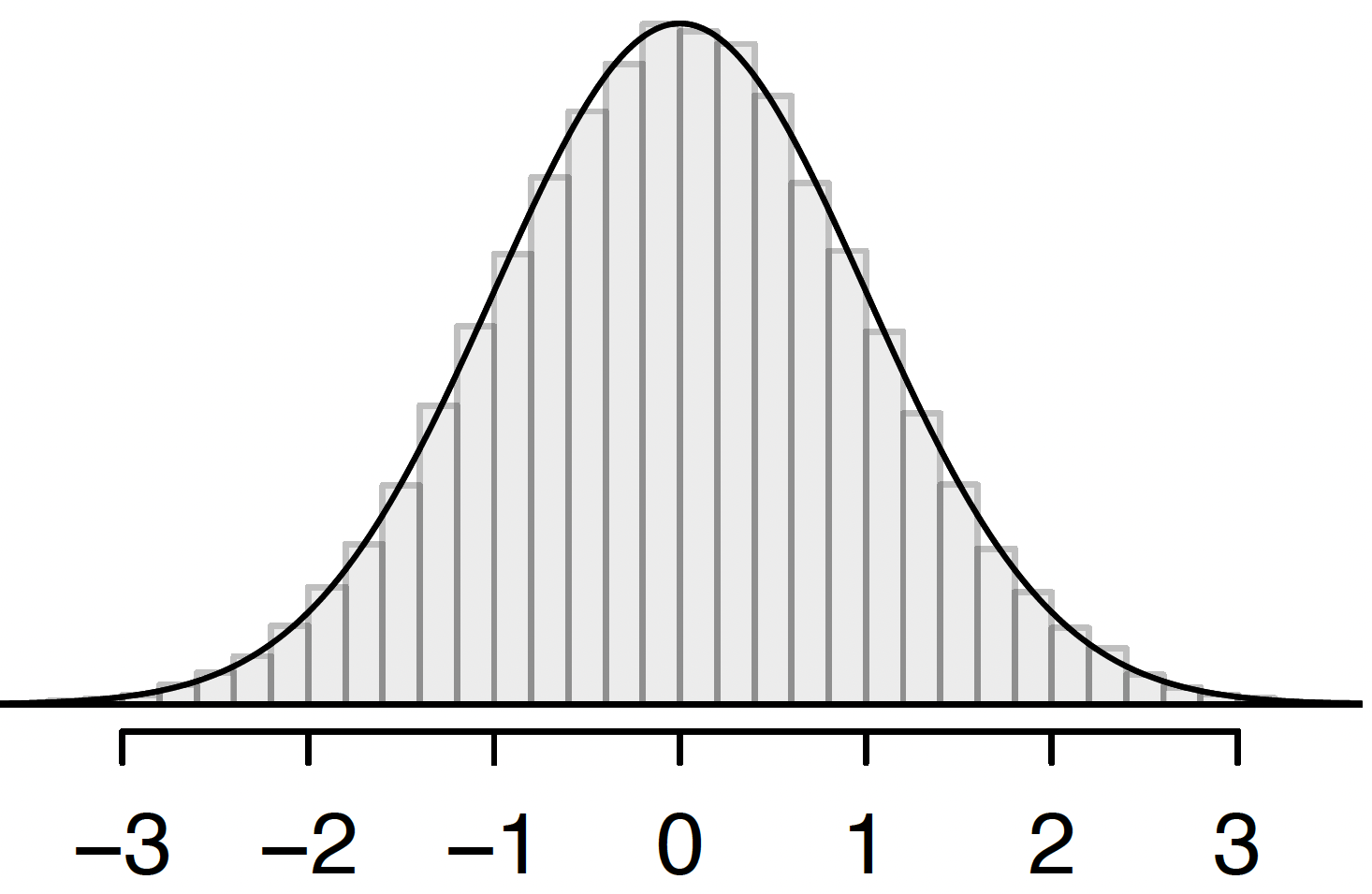
Standard Normal distribution (2/2)

Transformation from general normal \(X\) to standard normal \(Z\)

Normal distribution: R commands

R commands with their input and output:

R code	What does it return?
rnorm()	returns sample of random variables with specified normal distribution
dnorm()	returns value of probability density at certain point of the normal distribution Not typically used bc this is a continuous distributon
pnorm()	returns cumulative probability of getting certain point (or less) of the normal distribution
qnorm()	returns z-score corresponding to desired quantile

Calculating probabilities from a Normal distribution

Three ways to calculate probabilities from a normal distribution:

1. Calculus (not for us!)

 

2. Normal probability table

   • The textbook has a normal probability table in Appendix B.1, which is included as the next two pages
   • Not required for this class

 

3. R commands

   • \(P(Z \leq q) =\) pnorm(q, mean = 0, sd = 1, lower.tail = TRUE)

 

4. Random online calculators

   • Like this one: https://onlinestatbook.com/2/calculators/normal_dist.html

Example: Calculating probabilities from a Normal distribution (1/5)

Example: Calculating standard normal probabilities practice

Let \(Z\) be a standard normal random variable, \(Z\sim N(\mu=0,\sigma=1)\). Calculate the following probabilities. Include sketches of the normal curves with the probability areas shaded in.

1. \(\mathbb{P}( Z < 2.67 )\)

2. \(\mathbb{P}( Z > -0.37 )\)

3. \(\mathbb{P}( -2.18 < Z < 2.46 )\)

4. \(\mathbb{P}(Z = 1.53 )\)

Example: Calculating probabilities from a Normal distribution (2/5)

Example: Calculating standard normal probabilities practice

Let \(Z\) be a standard normal random variable, \(Z\sim N(\mu=0,\sigma=1)\). Calculate the following probabilities. Include sketches of the normal curves with the probability areas shaded in.

1. \(\mathbb{P}( Z < 2.67 )\)

1. Draw on standard Normal curve:

2. Calculate probability:

pnorm(q = 2.67, mean = 0, sd = 1)

[1] 0.9962074

pnorm(q = 2.67)

[1] 0.9962074

Example: Calculating probabilities from a Normal distribution (3/5)

Example: Calculating standard normal probabilities practice

Let \(Z\) be a standard normal random variable, \(Z\sim N(\mu=0,\sigma=1)\). Calculate the following probabilities. Include sketches of the normal curves with the probability areas shaded in.

2. \(\mathbb{P}( Z > -0.37 )\)

1. Draw on standard Normal curve:

1 - pnorm(q = -0.37, 
          mean = 0, 
          sd = 1)

[1] 0.6443088

pnorm(q = -0.37, mean = 0, sd = 1, 
      lower.tail = FALSE)

[1] 0.6443088

Example: Calculating probabilities from a Normal distribution (4/5)

Example: Calculating standard normal probabilities practice

Let \(Z\) be a standard normal random variable, \(Z\sim N(\mu=0,\sigma=1)\). Calculate the following probabilities. Include sketches of the normal curves with the probability areas shaded in.

3. \(\mathbb{P}( -2.18 < Z < 2.46 )\)

1. Draw on standard Normal curve:

pnorm(q = 2.46, mean = 0, sd = 1) - 
  pnorm(q = -2.18, mean = 0, sd = 1)

[1] 0.9784244

Example: Calculating probabilities from a Normal distribution (5/5)

Example: Calculating standard normal probabilities practice

Let \(Z\) be a standard normal random variable, \(Z\sim N(\mu=0,\sigma=1)\). Calculate the following probabilities. Include sketches of the normal curves with the probability areas shaded in.

4. \(\mathbb{P}(Z = 1.53 )\)

1. Draw on standard Normal curve:

Using Normal distribution in word problems

Example: Diastolic blood pressure (DBP)

Suppose the distribution of diastolic blood pressure (DBP) in 35- to 44-year old men is normally distributed with mean 80 mm Hg and variance 144 mm Hg.

1. Mild hypertension is when the DBP is between 90 and 99 mm Hg. What proportion of this population has mild hypertension?

2. What is the \(10^{th}\) percentile of the DBP distribution?

3. What is the \(95^{th}\) percentile of the DBP distribution?

Using Normal distribution in word problems

Example: Diastolic blood pressure (DBP)

Suppose the distribution of diastolic blood pressure (DBP) in 35- to 44-year old men is normally distributed with mean 80 mm Hg and variance 144 mm Hg.

1. Mild hypertension is when the DBP is between 90 and 99 mm Hg. What proportion of this population has mild hypertension?

• Draw on a normal curve:

• Compute in R:

pnorm(q = 99, mean = 80, 
      sd = sqrt(144)) - 
  pnorm(q = 90, mean = 80, 
        sd = sqrt(144))

[1] 0.1456556

Using Normal distribution in word problems

Example: Diastolic blood pressure (DBP)

Suppose the distribution of diastolic blood pressure (DBP) in 35- to 44-year old men is normally distributed with mean 80 mm Hg and variance 144 mm Hg.

2. What is the \(10^{th}\) percentile of the DBP distribution?

• Draw on a normal curve:

• Compute in R:

qnorm(p = 0.10, 
      mean = 80, 
      sd = sqrt(144))

[1] 64.62138

Using Normal distribution in word problems

Example: Diastolic blood pressure (DBP)

Suppose the distribution of diastolic blood pressure (DBP) in 35- to 44-year old men is normally distributed with mean 80 mm Hg and variance 144 mm Hg.

3. What is the \(95^{th}\) percentile of the DBP distribution?

• Draw on a normal curve:

• Compute in R:

qnorm(p = 0.95, 
      mean = 80, 
      sd = sqrt(144))

[1] 99.73824

Learning Objectives

1. Understand how probability distributions extend to continuous distributions
2. Calculate probabilities for specific events using a Normal distribution

3. Apply the Normal distribution to approximate probabilities for binomial events

4. Calculate probabilities for different events using a Poisson distribution

Normal Approximation of the Binomial Distribution

• Recall that a binomial random variable \(X\) counts the total number of successes in \(n\) independent trials, each with probability \(p\) of a success.

 

• Probability function for \(x = 0, 1, ..., n\) : \[P(X = k) = {n\choose k}p^k(1-p)^{n-k} = \frac{n!}{k!(n-k)!}p^k(1-p)^{n-k}\]

 

• Tedious to compute for large number of trails (\(n\)), although doable with software like R

 

• As \(n\) gets big though, the distribution shape of a binomial r.v. gets more and more symmetric, and can be approximated by a normal distribution

• Pretty good video behind the intuition of this (Watch 00:00 - 05:40)

We can look at a plot of Binomial distributions

• Binomial distributions for different \(n\) (columns) and \(p\) (rows)

Normal Approximation of the Binomial Distribution

• Also known as: Sampling distribution of \(\widehat{p}\)

• If \(X\sim \text{Binomial}(n,p)\) and \(np>10\) and \(nq = n(1-p) > 10\)

  • Ensures sample size (\(n\)) is moderately large and the \(p\) is not too close to 0 or 1
  • Other resources use other criteria (like \(npq>5\) or \(np>5\))

 

• THEN approximately \[X\sim \text{Normal}\big(\mu_X = np, \sigma_X = \sqrt{np(1-p)} \big)\]

• Continuity Correction: Applied to account for the fact that the binomial distribution is discrete, while the normal distribution is continuous

  • Adjust the binomial value (# of successes) by ±0.5 before calculating the normal probability.
  • For \(P(X \leq k)\) (Binomial), you would instead calculate \(P(X \leq k + 0.5)\) (Normal approx)
  • For \(P(X \geq k)\) (Binomial), you would instead calculate \(P(X \leq k - 0.5)\) (Normal approx)

Example: Normal approximation or Binomial distribution (1/2)

Example: Vaccinated people testing positive for Covid-19 (revisited)

About 25% of people that test positive for Covid-19 are vaccinated for it. Suppose 100 people have tested positive for Covid-19 (independently of each other). Let \(X\) denote the number of people that are vaccinated among the 100 that tested positive. What is the probability that fewer than 20 of the people that tested positive are vaccinated?

1. Calculate exact probability.

2. Calculate approximate probability.

\(p=0.25\), \(n=100\), we want \(P(X < 20)\)

 

1. Exact probability = Binomial distribution

\[X \sim \text{Binomial}(n=100, p=0.25)\]

\[P(X < 20) = P(X \leq 19) = \sum_{j=0}^{19}P(X = j)\]

 

pbinom(q = 19, size = 100, prob = 0.25)

[1] 0.09953041

Example: Normal approximation or Binomial distribution (2/2)

Example: Vaccinated people testing positive for Covid-19 (revisited)

About 25% of people that test positive for Covid-19 are vaccinated for it. Suppose 100 people have tested positive for Covid-19 (independently of each other). Let \(X\) denote the number of people that are vaccinated among the 100 that tested positive. What is the probability that fewer than 20 of the people that tested positive are vaccinated?

1. Calculate exact probability.

2. Calculate approximate probability.

\(p=0.25\), \(n=100\), we want \(P(X < 20)\)

2. Approximate probability = Normal distribution

   • Mean = \(\mu = np = 0.25\cdot 100 = 25\)
   • SD = \(\sigma = \sqrt{np(1-p)}=\sqrt{100\cdot 0.25 \cdot (1-0.25)} = 4.33\)

\[X \sim \text{Normal}\big(\mu=25, \sigma = 4.33\big)\]

• Use continuity correction: Instead of calculating \(P(X \leq 19)\), we calculate \(P(X \leq 19.5)\)

pnorm(q = 19.5, mean = 25, 
      sd = sqrt( 100*0.25*0.75 ))

[1] 0.1020119

Some resources for the normal distribution

• Page on R commands

Learning Objectives

1. Understand how probability distributions extend to continuous distributions
2. Calculate probabilities for specific events using a Normal distribution
3. Apply the Normal distribution to approximate probabilities for binomial events

4. Calculate probabilities for different events using a Poisson distribution

Introduction to the Poisson distribution

• The Poisson distribution is often used to model count data (# of successes), especially for rare events

  • It is a discrete distribution!

 

• It is used most often in settings where events happen at a rate \(\lambda\) per unit of population and per unit time

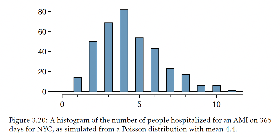
• Example: historical records of hospitalizations in New York City indicate that an average of 4.4 people are hospitalized each day for an acute myocardial infarction (AMI)

  • We can plot the distribution of hospitalizations on each day

 

Poisson distribution

• Suppose events occur over time in such a way that

  1. The probability an event occurs in an interval is proportional to the length of the interval.

  2. Events occur independently at a rate \(\lambda\) per unit of time.

• Then the probability of exactly \(x\) events in one unit of time is \[ P(X = k) = \frac{e^{-\lambda}\lambda^{k}}{k!}, \,\, k = 0, 1, 2, \ldots \]

• For the Poisson distribution modeling the number of events in one unit of time:

  • The mean is \(\lambda\).

  • The standard deviation is \(\sqrt{\lambda}\).

• Shorthand for a random variable, \(X\), that has a Poisson distribution: \[X \sim \text{Pois}(\lambda)\]

Poisson distribution: R commands

R commands with their input and output:

R code	What does it return?
rpois()	returns sample of random variables with specified Poisson distribution
dpois()	returns value of probability density at certain point of the Poisson distribution
ppois()	returns cumulative probability of getting certain point (or less) of the Poisson distribution
qpois()	returns number of cases corresponding | to desired quantile

Example: probabilities from a Poisson distribution (1/4)

Typhoid fever

Suppose there are on average 5 deaths per year from typhoid fever over a 1-year period.

1. What is the probability of 3 deaths in a year?

2. What is the probability of 2 deaths in 0.5 years?

3. What is the probability of more than 12 deaths in 2 years?

Example: probabilities from a Poisson distribution (2/4)

Typhoid fever

Suppose there are on average 5 deaths per year from typhoid fever over a 1-year period.

1. What is the probability of 3 deaths in a year?

• \(\lambda = 5\) and we want \(P(X = 3)\)

\[P(X=3) = \frac{e^{-5}5^{3}}{3!} = 0.1404\]

dpois(x = 3, lambda = 5)

[1] 0.1403739

Example: probabilities from a Poisson distribution (3/4)

Typhoid fever

Suppose there are on average 5 deaths per year from typhoid fever over a 1-year period.

2. What is the probability of 2 deaths in 0.5 years?

\(\lambda = ?\) and we want \(P(X = 2)\)

• \(\lambda=5\) was the rate for one year. When we want the rate for half year, we need to calculate a new \(\lambda\):

  • \(\lambda = \dfrac{5 \text{ deaths}}{1 \text{ year}}\cdot\dfrac{1 \text{ year}}{2 \text{ half-years}}=\dfrac{2.5 \text{ deaths}}{1 \text{ half-year}}\)

\[P(X=2) = \frac{e^{-2.5}2.5^{2}}{2!} = 0.0.2565\]

dpois(x = 2, lambda = 2.5)

[1] 0.2565156

Example: probabilities from a Poisson distribution (4/4)

Typhoid fever

Suppose there are on average 5 deaths per year from typhoid fever over a 1-year period.

3. What is the probability of more than 12 deaths in 2 years?

\(\lambda = ?\) and we want \(P(X > 12)\)

• Need to calculate a new \(\lambda\) for 2 years: \(\lambda = \dfrac{5 \text{ deaths}}{1 \text{ year}}\cdot\dfrac{2 \text{ years}}{1 \text{ two-years}}=\dfrac{10 \text{ deaths}}{1 \text{ two-year}}=\dfrac{10 \text{ deaths}}{2 \text{ years}}\)

\[P(X>12) = 1 - P(X \leq 12) = 1 - \sum_{k=0}^{12}\frac{e^{-10}10^{k}}{k!} = 0.2084\]

1 - ppois(q = 12, lambda = 10)

[1] 0.2084435

ppois(q = 12, lambda = 10, 
      lower.tail = F)

[1] 0.2084435

Poisson approximation of binomial distribution

• Poisson distribution can be used to approximate binomial distribution when \(n\) is large and \(p\) is small
  • When Normal approximation does not work
• Binomial distributions for different \(n\) (columns) and \(p\) (rows)