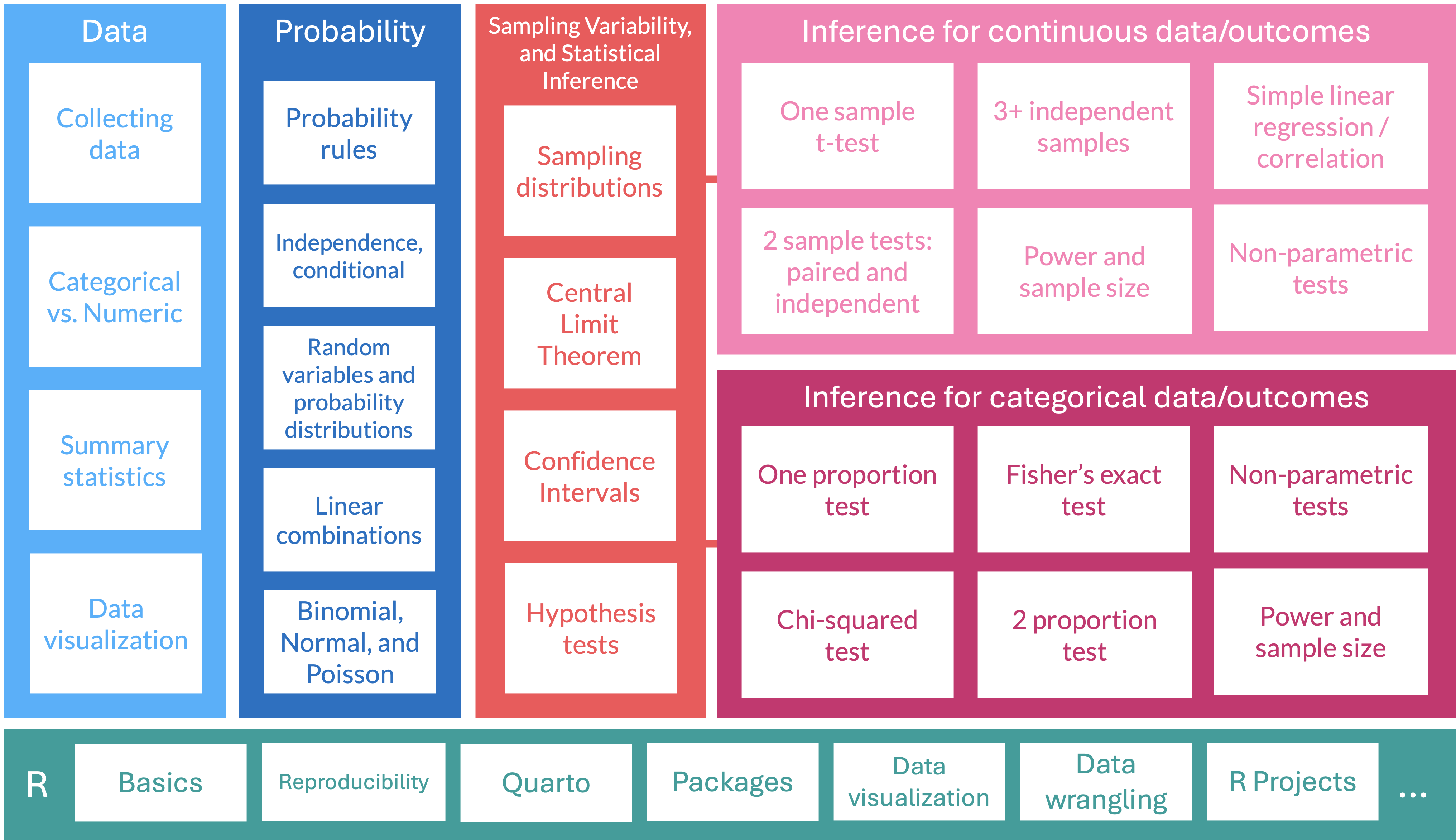
Lesson 9: Variability in estimates

TB sections 4.1

Nicky Wakim

2024-10-30

Artwork by @allison_horst

Learning Objectives

Illustrate how information from several samples are connected to the population and to the sampling distribution
Understand how the sampling distribution of the sample means relates to a sample and the population distribution
Apply the Central Limit Theorem to approximate the sampling distribution of the sample mean

Where are we?

From Lesson 1: Population vs. sample

(Target) Population

Group of interest being studied
Group from which the sample is selected
- Studies often have inclusion and/or exclusion criteria
Almost always too expensive or logistically impossible to collect data for every case in a population

Sample

Group on which data are collected
Often a small subset of the population
Easier to collect data on
If we do it right, we might be able to answer our question about the target population

Goal is to get a representative sample of the population: the characteristics of the sample are similar to the characteristics of the population

Why sample statistics?

When we want to estimate features of the population
- We can use corresponding summary statistics calculated from our sample
- Often called point estimates or sample statistics

Much easier to measure statistics from our sample (Lesson 1)
- However, statistics from our sample are not exactly the same as the population measurements that we’re aiming for
- We call the population measurements population parameters

So we need to start by distinguishing between the population parameters and sample statistics

Population parameters vs. sample statistics

Population parameter

Mean: \(\mu\) (“mu”)
Standard deviation: \(\sigma\) (“sigma”)
Variance: \(\sigma^2\)

Proportion: \(p\), \(\pi\) (“pi”)

Correlation

Sample statistic (point estimate)

Sample mean: \(\overline{x}\)
Sample standard deviation: \(s\)
Sample variance: \(s^2\)

Sample proportion: \(\hat{p}\) (“p-hat”)

Sample correlation coefficient: \(r\)

Poll Everywhere Question 1

Learning Objectives

Illustrate how information from several samples are connected to the population and to the sampling distribution

Understand how the sampling distribution of the sample means relates to a sample and the population distribution
Apply the Central Limit Theorem to approximate the sampling distribution of the sample mean

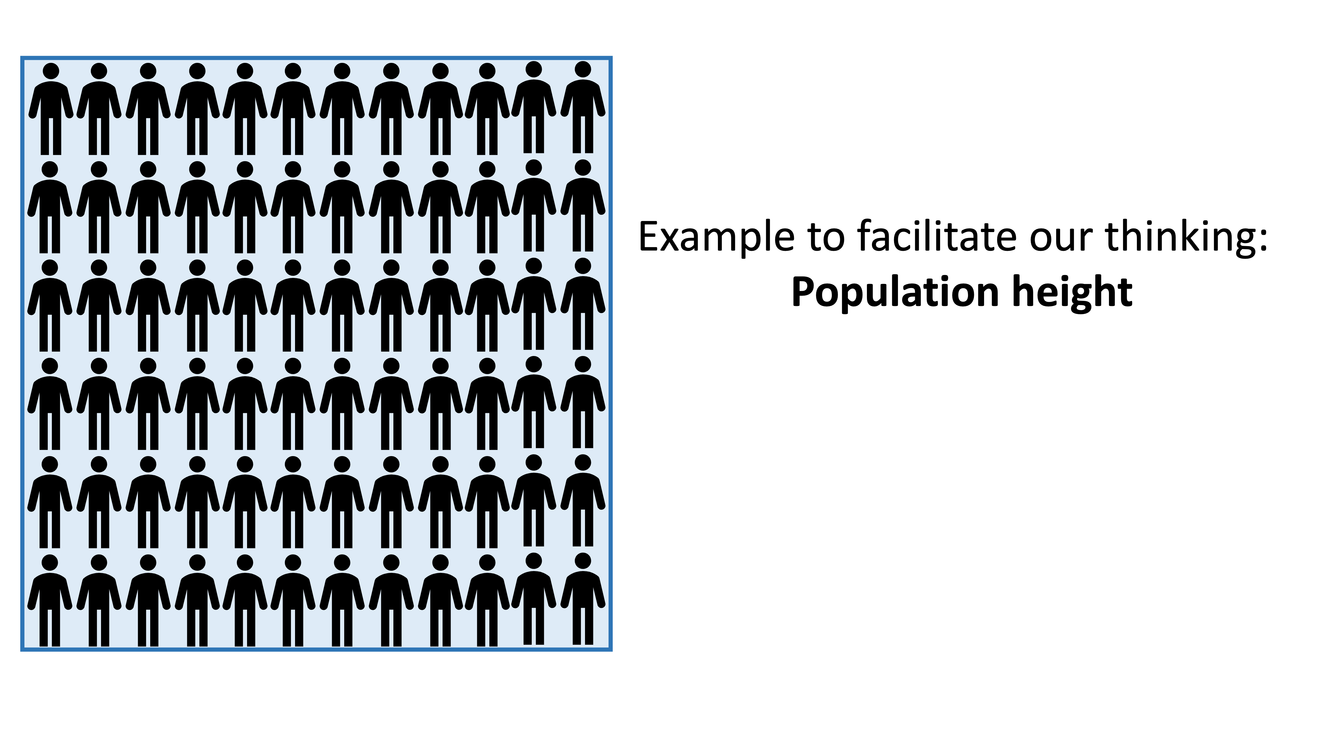
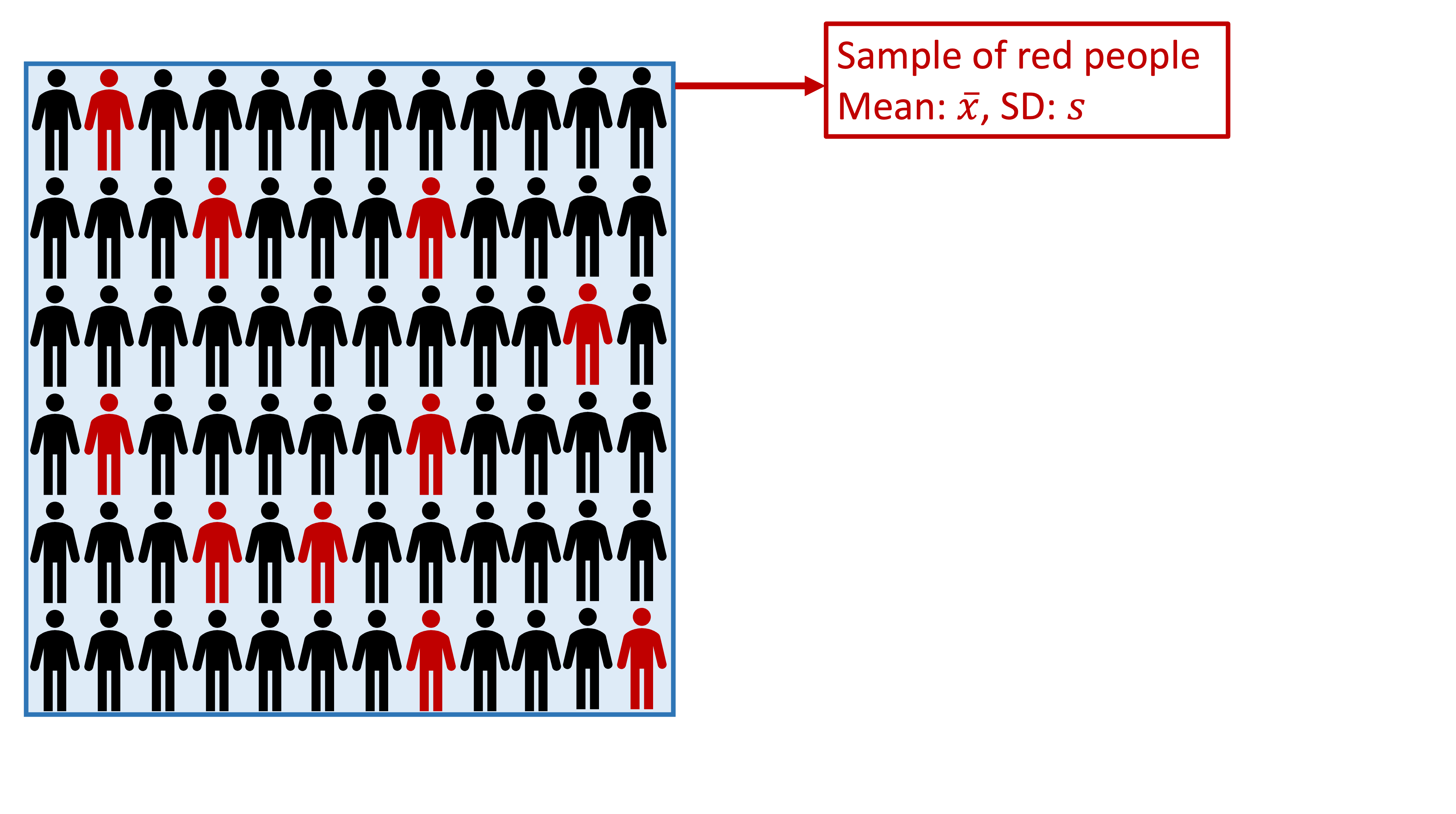
Population

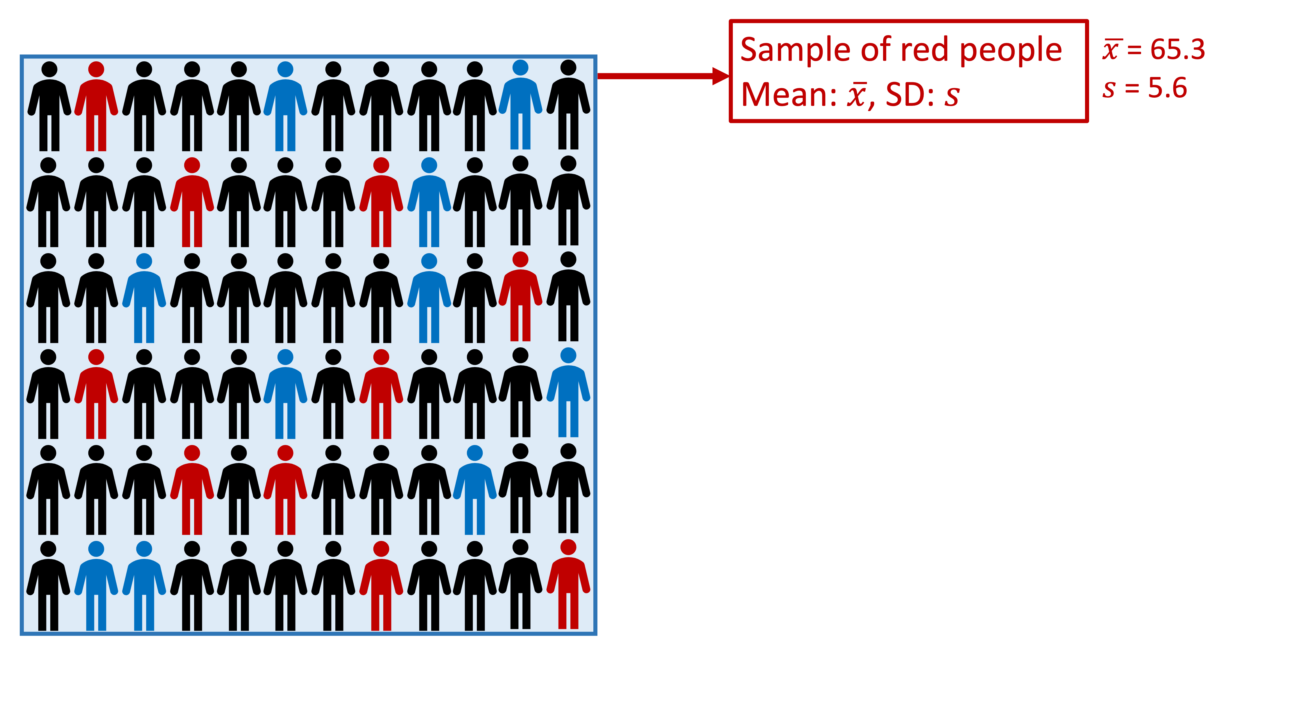
Take one sample

Take another sample

Poll Everywhere Question 2

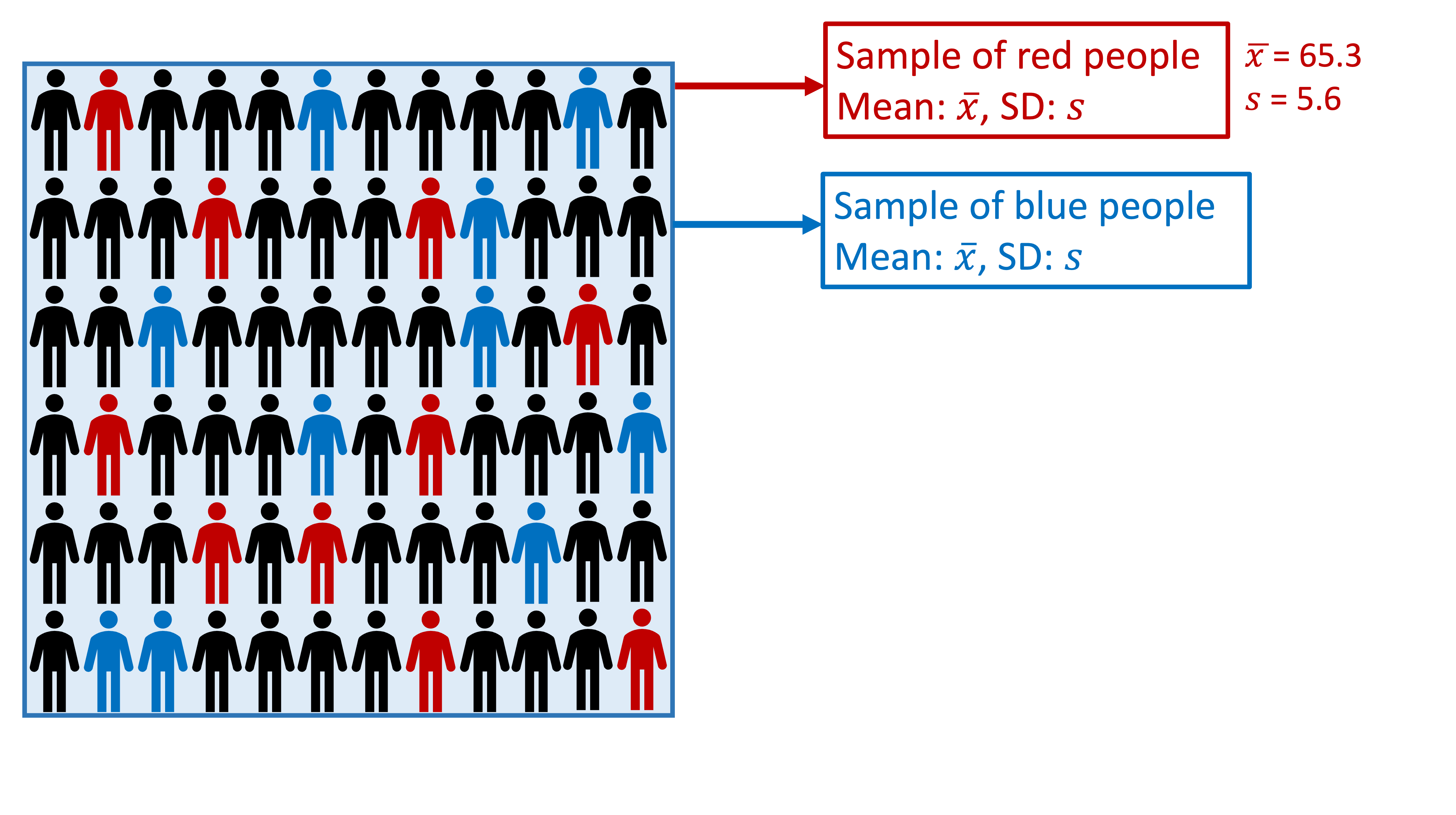
Take another sample

Take several samples

Difference between samples?

Learning Objectives

Illustrate how information from several samples are connected to the population and to the sampling distribution

Understand how the sampling distribution of the sample means relates to a sample and the population distribution

Apply the Central Limit Theorem to approximate the sampling distribution of the sample mean

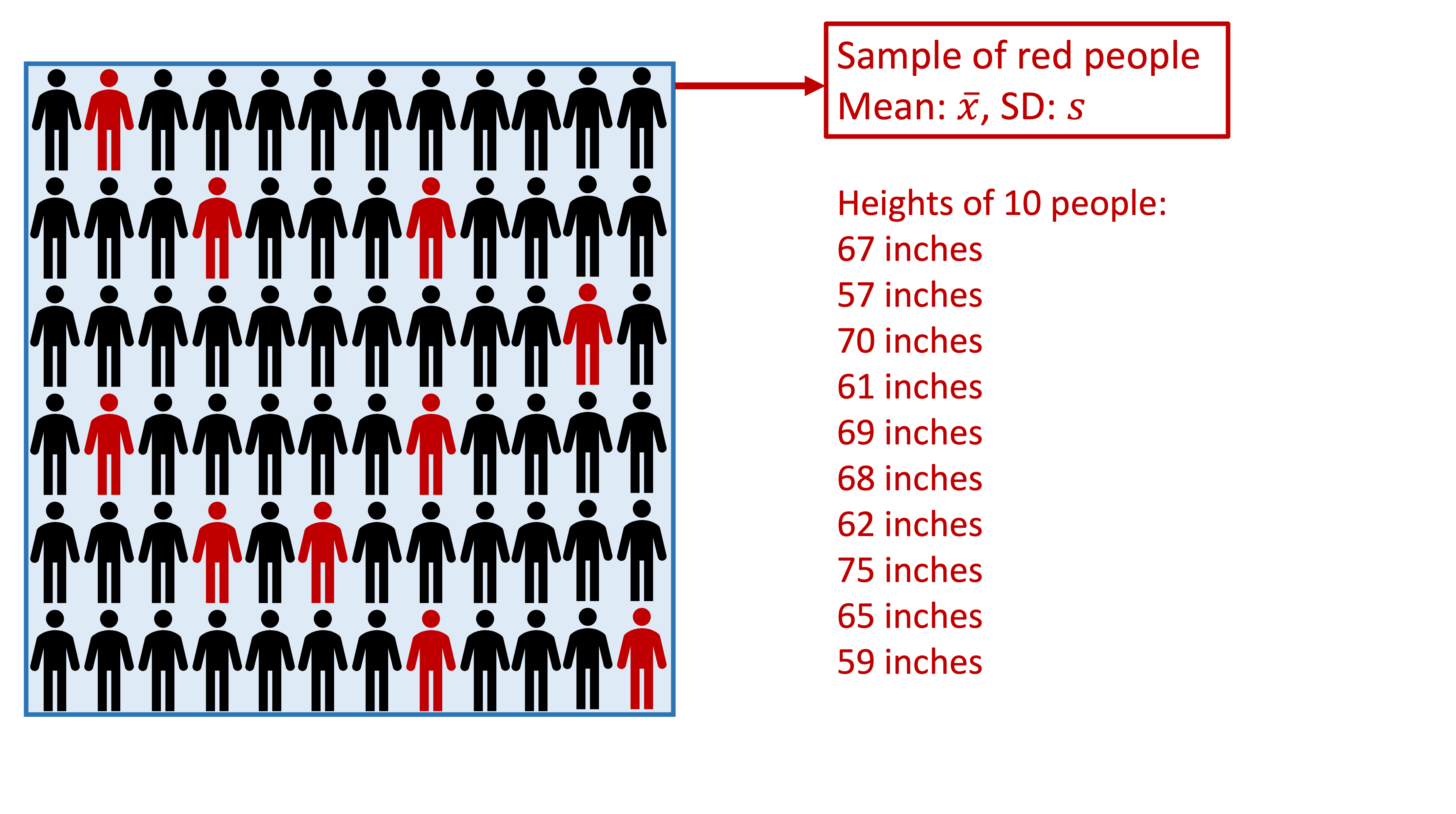
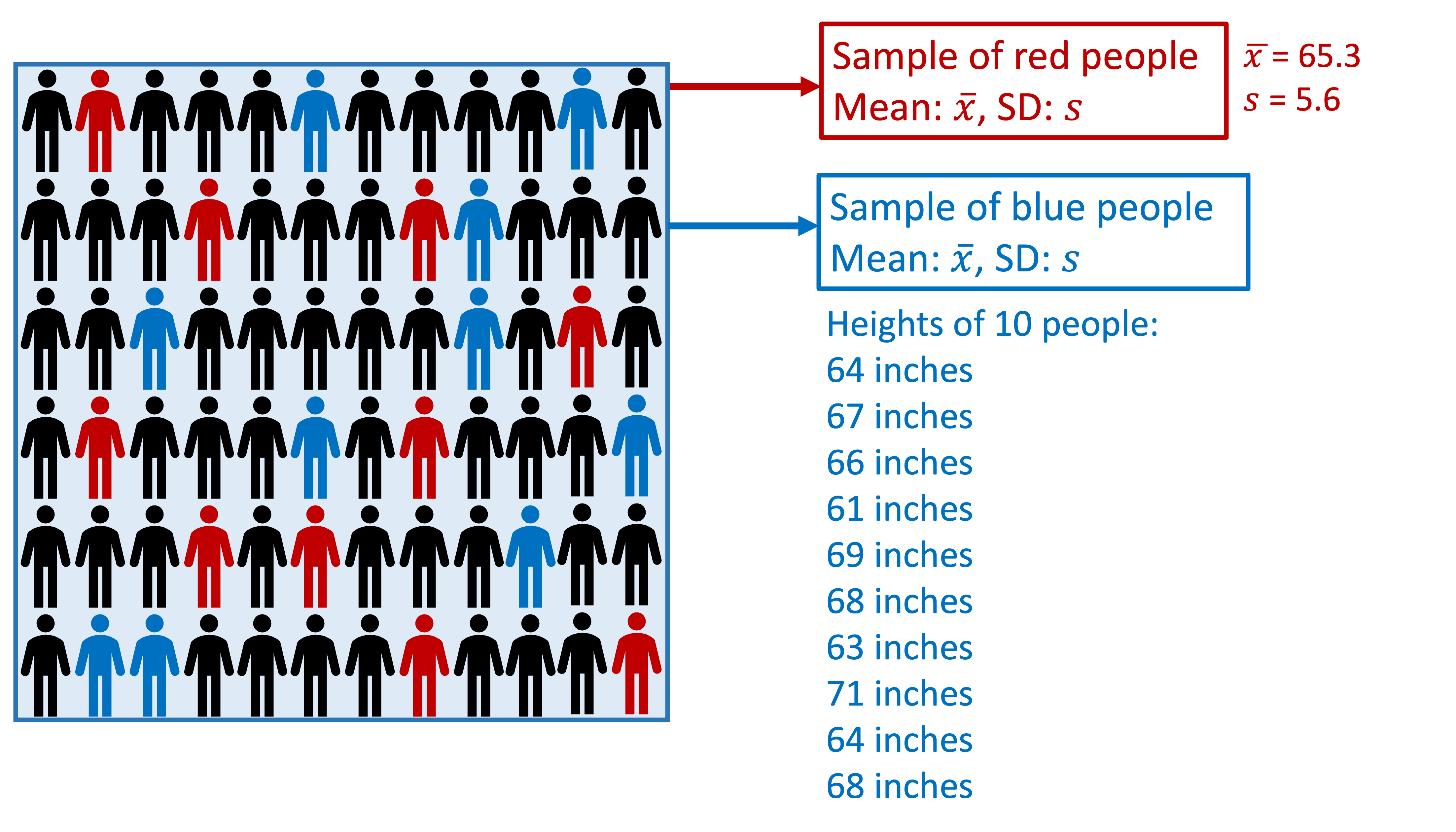
More concrete example with height (1/3)

Variation in population (\(\sigma\)):

\[ \mu = 65 \text{ inches}\] \[ \sigma = 3 \text{ inches}\]

More concrete example with height (2/3)

Variation in population (\(\sigma\)):

\[ \mu = 65 \text{ inches}\] \[ \sigma = 3 \text{ inches}\]

Variation within samples (\(s\)):

More concrete example with height (3/3)

Variation in population (\(\sigma\)):

\[ \mu = 65 \text{ inches}\] \[ \sigma = 3 \text{ inches}\]

Variation within samples (\(s\)):

Variation between samples (\(SE\)):

\[ \mu_{\overline{X}} = 65.002 \text{ inches}\] \[ SE = 0.421 \text{ inches}\]

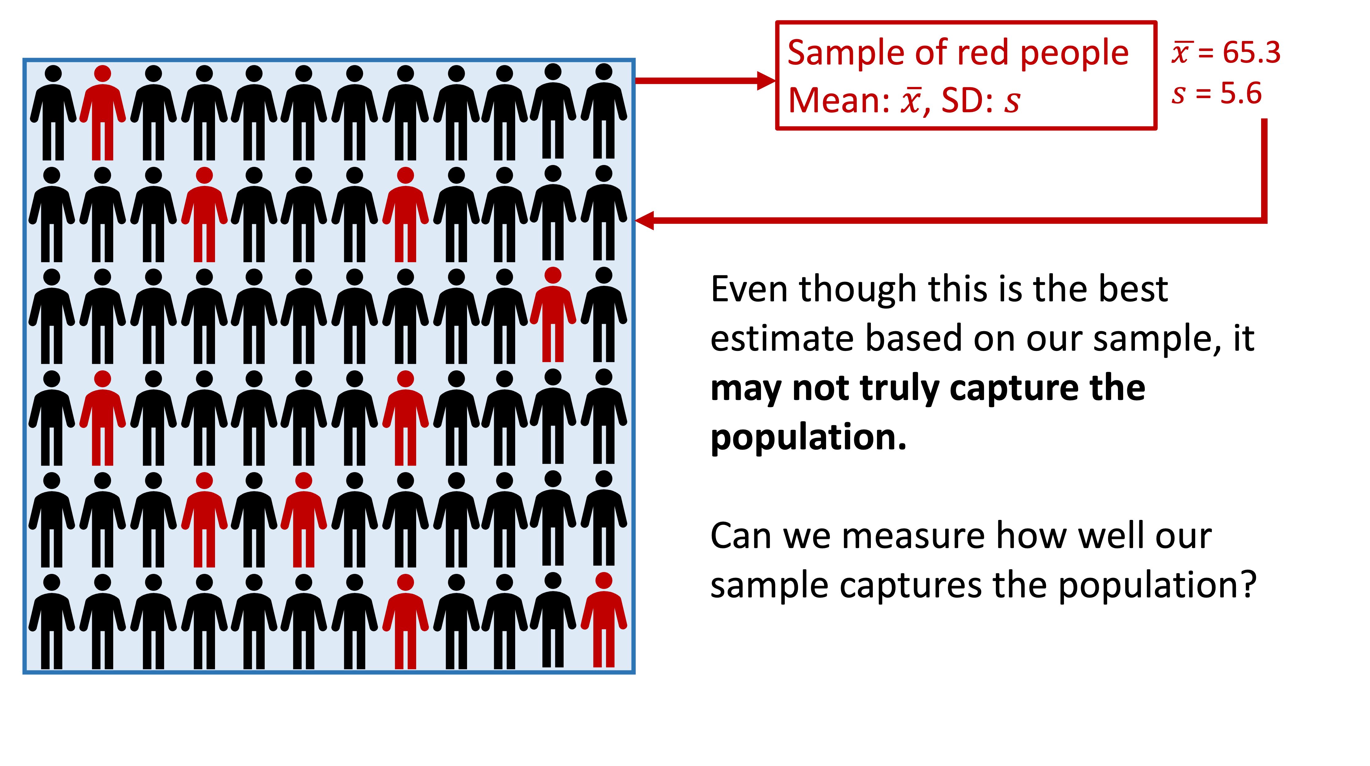
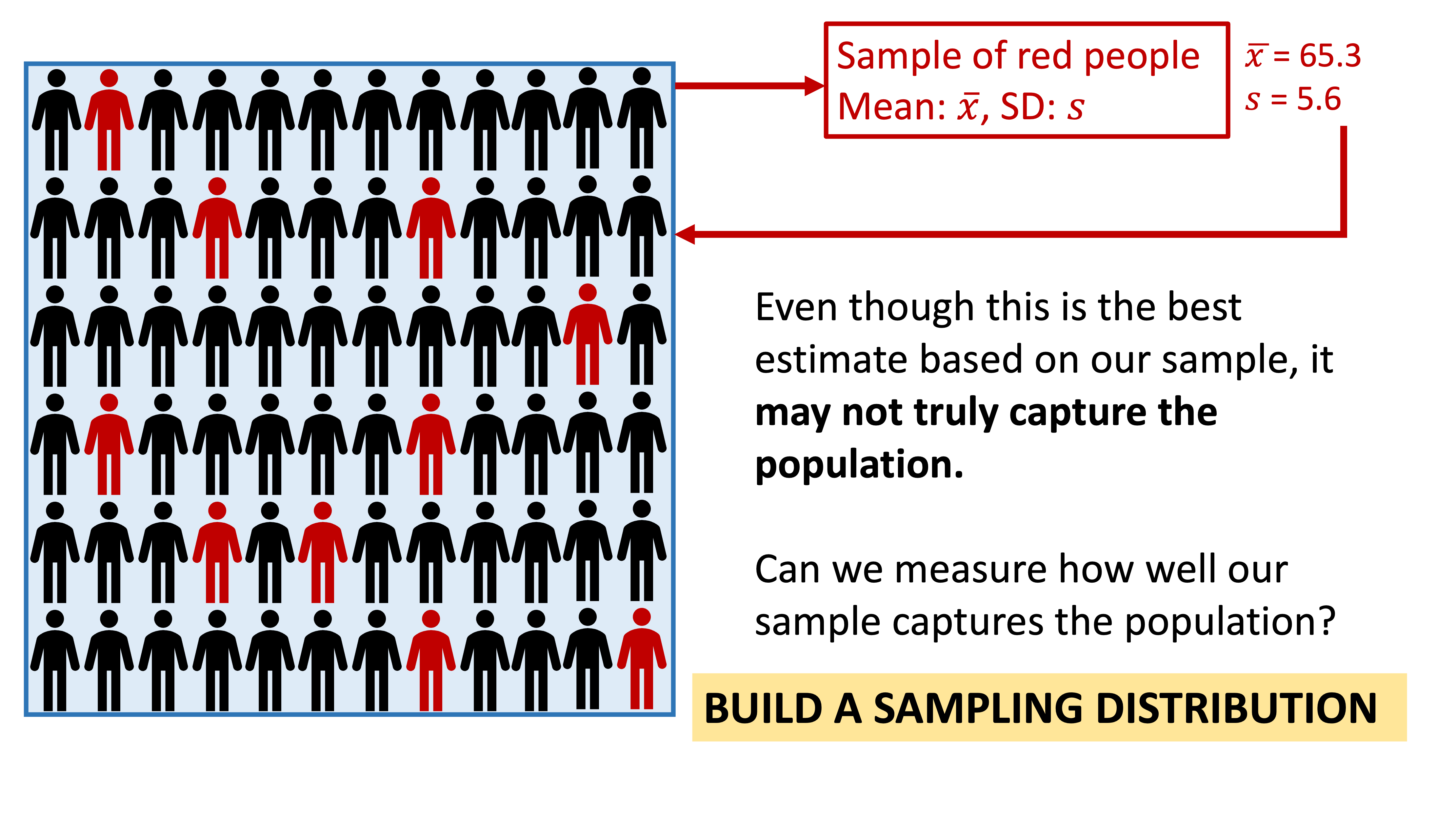
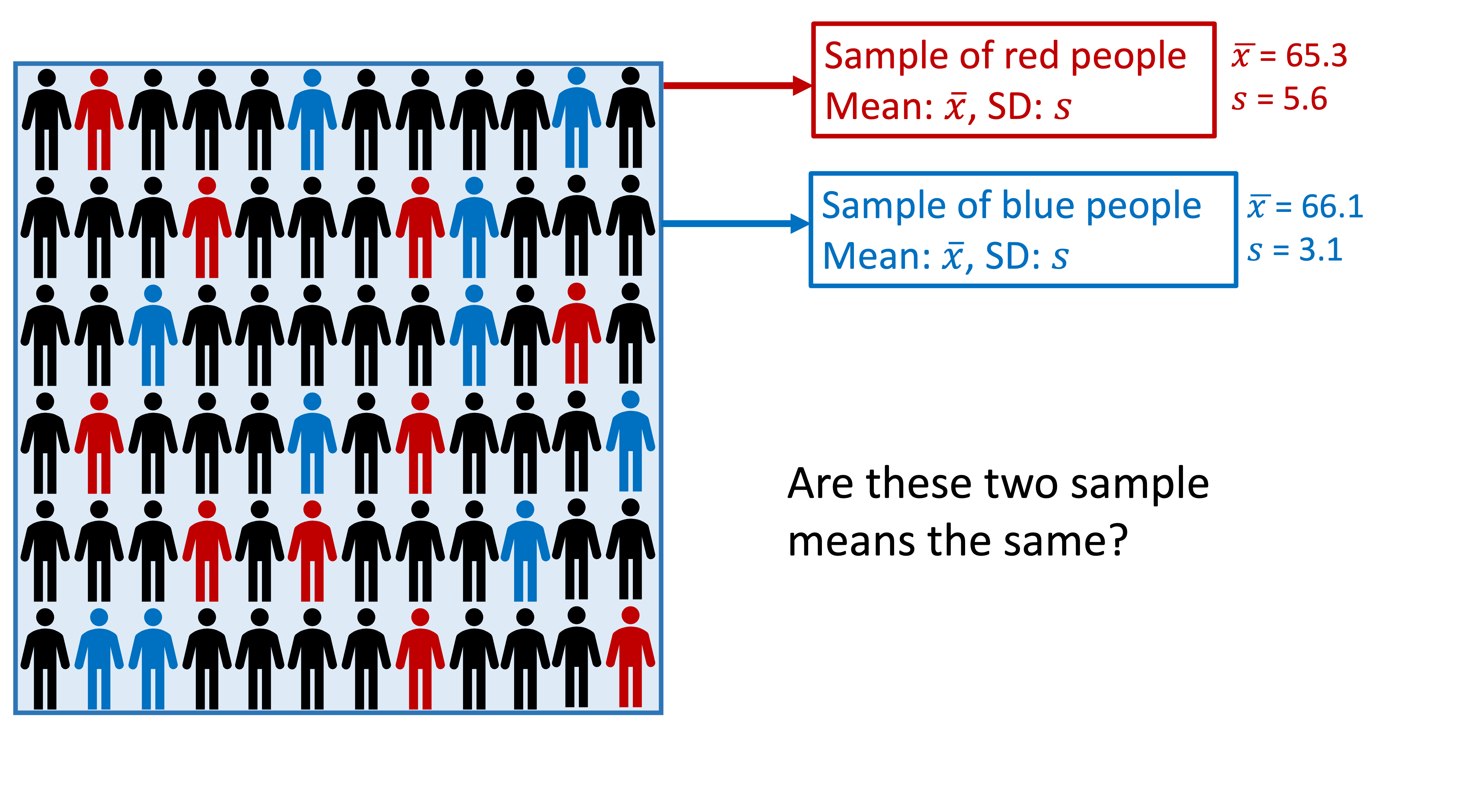
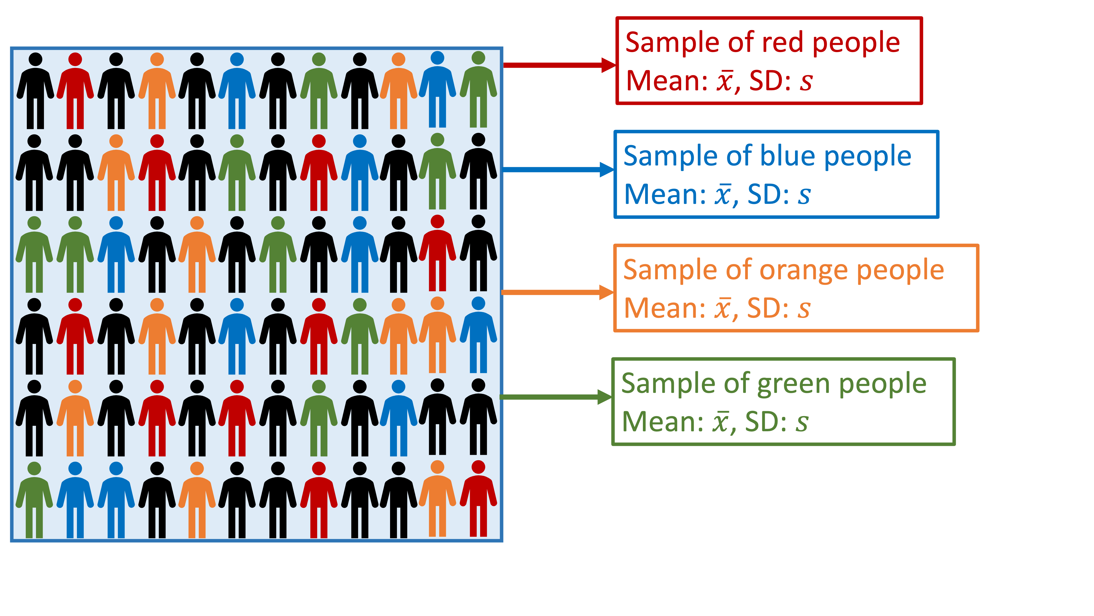
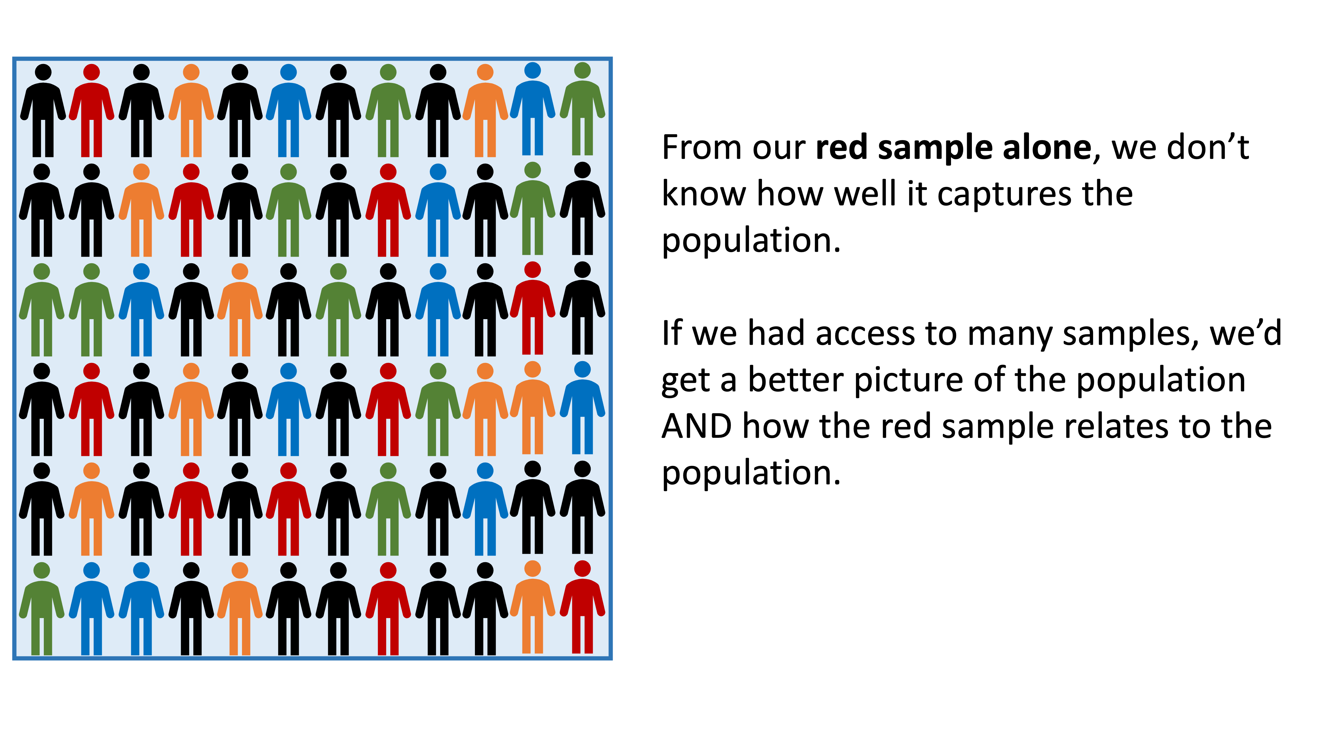
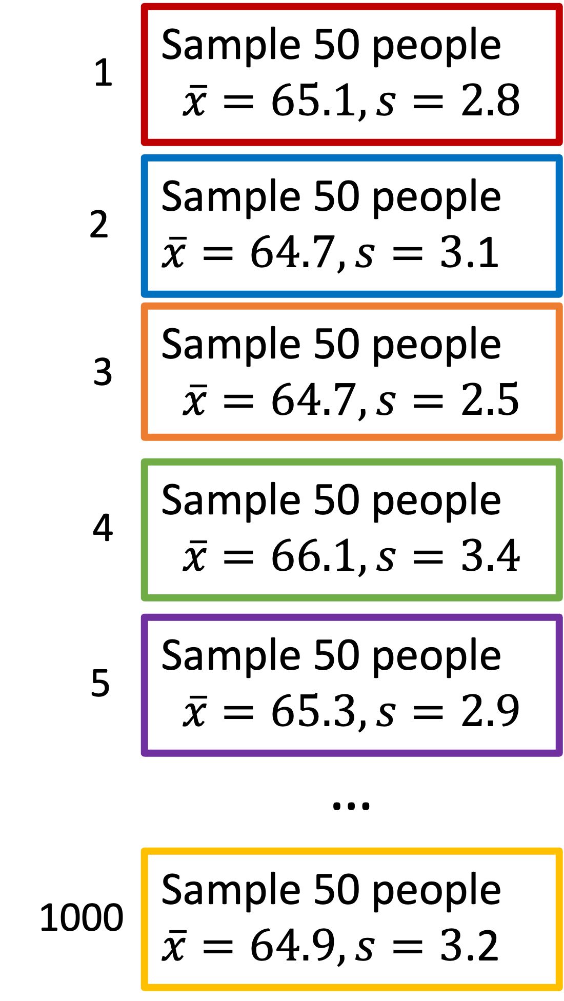
Sampling Distribution of Sample Means

The sampling distribution is the distribution of sample means calculated from repeated random samples of the same size from the same population
It is useful to think of a particular sample statistic as being drawn from a sampling distribution
- So the red sample with \(\overline{x} = 65.1\) is just one sample mean in the sampling distribution

Variation between samples (\(SE\)):

\[ \mu_{\overline{X}} = 65.002 \text{ inches}\] \[ SE = 0.421 \text{ inches}\]

For following Poll Everywhere Question

How are the center, shape, and spread similar and/or different?

Poll Everywhere Question 3

Okay, but in real life we only have one sample…?

In a study, conclusions about a population parameter must be drawn from the data collected from a single sample

The sampling distribution of \(\overline{X}\) is a theoretical concept
- Obtaining repeated samples by conducting a study many times is not possible

Not feasible to calculate the population mean \(\mu\) by finding the mean of the sampling distribution for \(\overline{X}\)

In the next lesson on confidence intervals, we’ll see what kind of statements we can make about the population mean from a single sample

Learning Objectives

Illustrate how information from several samples are connected to the population and to the sampling distribution
Understand how the sampling distribution of the sample means relates to a sample and the population distribution

Apply the Central Limit Theorem to approximate the sampling distribution of the sample mean

The Central Limit Theorem (CLT)

If a sample consists of at least 30 independent observations, then the sampling distribution of the sample mean is approximated by a normal model
Aka, for “large” sample sizes ( \(n\geq 30\) ),
- The sampling distribution of the sample mean can be approximated by a normal distribution,with
  - Mean equal to the population mean value \(\mu\)
  - Standard deviation \(\frac{\sigma}{\sqrt{n}}\)
This is regardless of the original sample is from a different distribution
- For example, if we count the number of heads in 50 coin flips, and do this for many samples, then our sampling distribution will be Normally distributed around \(n\cdot p = 50 \cdot 0.5= 25\)

Other cases for normal approximation

For small sample sizes, if the population is known to be normally distributed, then
- The sampling distribution of the sample mean is a normal distribution, with
  - Mean equal to the population mean value \(\mu\), and
  - Standard deviation \(\frac{\sigma}{\sqrt{n}}\)
Not technically the Central Limit Theorem, but sampling distribution approximated using same Normal distribution

Sampling Distribution of Sample Means (with the CLT)

The sampling distribution is the distribution of sample means calculated from repeated random samples of the same size from the same population
It is useful to think of a particular sample statistic as being drawn from a sampling distribution
- So the red sample with \(\overline{x} = 65.1\) is just one sample mean in the sampling distribution

With CLT and \(\overline{X}\) as the RV for the sampling distribution

Theoretically (using only population values): \(\overline{X} \sim \text{Normal} \big(\mu_{\overline{X}} = \mu, \sigma_{\overline{X}}= SE = \frac{\sigma}{\sqrt{n}} \big)\)
In real use (using sample values for SE): \(\overline{X} \sim \text{Normal} \big(\mu_{\overline{X}} = \mu, \sigma_{\overline{X}}= SE = \frac{s}{\sqrt{n}} \big)\)

Variation between samples (\(SE\)):

\[ \mu_{\overline{X}} = 64.996 \text{ inches}\] \[ SE = 0.291 \text{ inches}\]

Let’s apply the CLT to our sampling distribution when n = 50 (1/2)

CLT tells us that we can model the sampling distribution of mean heights using a normal distribution:

Let’s apply the CLT to our sampling distribution when n = 50 (2/2)

Mean and SD of population: \[ \mu = 65 \text{ inches} \text{, } \sigma = 3 \text{ inches}\]

From the CLT, we can figure out the theoretical mean and standard deviation of our sampling distribution:

\[ \mu = 65 \text{ inches}\] \[ SE = \frac{\sigma}{\sqrt{n}} \text{ inches} = \frac{3}{\sqrt{50}} \text{ inches} = 0.424 \text{ inches}\]

I simulated the data, so I can calculate mean and SE of the sampling distribution:

(sample_mean = mean(means50$means))

[1] 65.00198

(sample_se = sd(means50$means))

[1] 0.4212266

Applying the CLT (1/2)

Example 1

For a random sample of 100 people, what is the probability that their mean height is greater than 65 inches? We happen to know the population mean is 64 inches and population standard deviation is 4 inches.

Make sure that the number of individuals in the sample is greater than 30: \(100 > 30\), so we can use the CLT
Find the mean and standard error for our sampling distribution: \[\mu_{\overline{X}}=64\] \[SE = \frac{\sigma}{\sqrt{n}}= \frac{4}{\sqrt{100}}= 0.4 \text{ inches}\] \[ \overline{X} \sim \text{Normal} (64, 0.4)\]

Applying the CLT (2/2)

Example 1

Calculate the probability from a Normal distribution: \(P(H \geq 65)\)

pnorm(q = 65, mean = 64, sd = 0.4, 
      lower.tail = F)

[1] 0.006209665

The probability that a 100-person sample has a mean of 65 or greater is 0.006. Makes me question if our sample really came from the population…

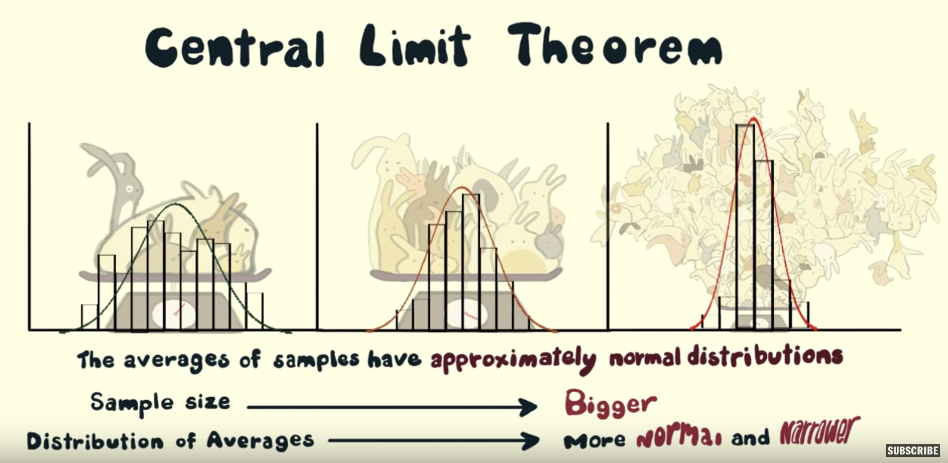
Check out this video explanation of CLT

Bunnies, Dragons and the ‘Normal’ World: Central Limit Theorem
- Creature Cast from the New York Times
- https://www.youtube.com/watch?v=jvoxEYmQHNM&feature=youtu.be

Summary Review: Point Estimate Terminology

Population mean: \(\mu\)
Population standard deviation: \(\sigma\)
Sample mean: \(\overline{x}\)
Sample standard deviation: \(s\)
Sampling distribution: Distribution of sample means for repeated samples.
- Use \(\overline{X}\) as the RV for this distribution
- \(\overline{X} \sim \text{Normal} \bigg(\mu_{\overline{X}} = \mu, \sigma_{\overline{X}}= SE = \frac{s}{\sqrt{n}} \bigg)\)
Standard error (SE): The standard deviation of the sampling distribution.
- Formula: \(SE = \frac{s}{\sqrt{n}}\)