Lesson 13: Inference for difference in means from two independent samples

TB sections 5.3

Meike Niederhausen and Nicky Wakim

2024-11-13

Learning Objectives

Identify when a research question or dataset requires two independent sample inference.
Construct and interpret confidence intervals for difference in means of two independent samples.
Run a hypothesis test for two sample independent data and interpret the results.

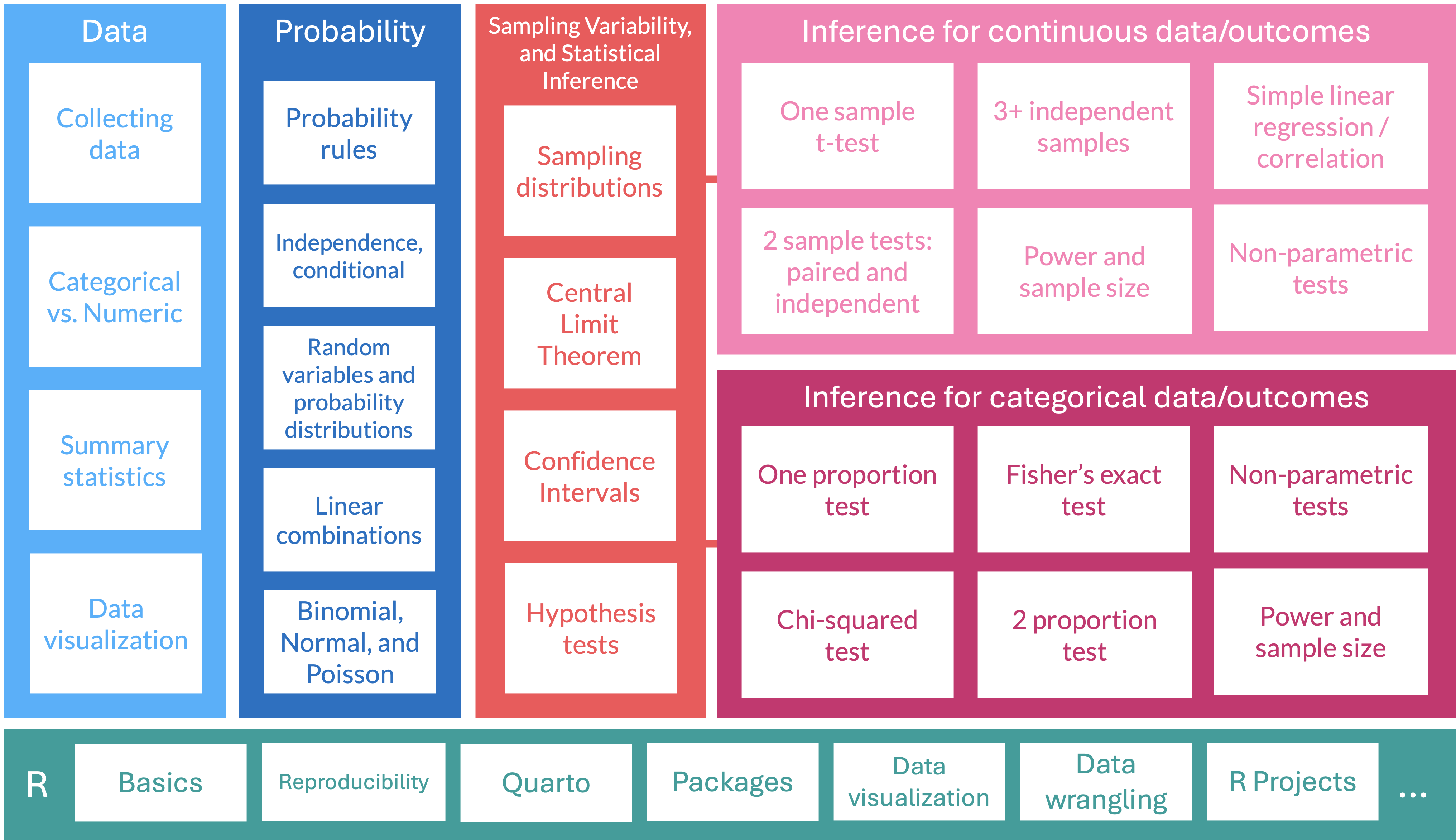
Where are we?

Different types of inference based on different data types

Lesson	Section	Population parameter	Symbol (pop)	Point estimate	Symbol (sample)	SE
11	5.1	Pop mean	\(\mu\)	Sample mean	\(\overline{x}\)	\(\dfrac{s}{\sqrt{n}}\)
12	5.2	Pop mean of paired diff	\(\mu_d\) or \(\delta\)	Sample mean of paired diff	\(\overline{x}_{d}\)	\(\dfrac{s_d}{\sqrt{n}}\)
13	5.3	Diff in pop means	\(\mu_1-\mu_2\)	Diff in sample means	\(\overline{x}_1 - \overline{x}_2\)	????
15	8.1	Pop proportion	\(p\)	Sample prop	\(\widehat{p}\)
15	8.2	Diff in pop prop’s	\(p_1-p_2\)	Diff in sample prop’s	\(\widehat{p}_1-\widehat{p}_2\)

Learning Objectives

Identify when a research question or dataset requires two independent sample inference.

Construct and interpret confidence intervals for difference in means of two independent samples.
Run a hypothesis test for two sample independent data and interpret the results.

What are data from two independent sample?

Two independent samples: Individuals between and within samples are independent
- Typically: measure the same outcome for each sample, but typically the two samples differ based on a single variable

Examples
- Any study where participants are randomized to a control and treatment group
- Study with two groups based on their exposure to some condition (can be observational)
- Book: “Does treatment using embryonic stem cells (ESCs) help improve heart function following a heart attack?”
- Book: “Is there evidence that newborns from mothers who smoke have a different average birth weight than newborns from mothers who do not smoke?”

Pairing (like comparing before and after) may not be feasible

Poll Everywhere Question 1

For two independent samples: Population parameters vs. sample statistics

Population parameter

Population 1 mean: \(\mu_1\)
Population 2 mean: \(\mu_2\)

Difference in means: \(\mu_1 - \mu_2\)

Population 1 standard deviation: \(\sigma_1\)
Population 2 standard deviation: \(\sigma_2\)

Sample statistic (point estimate)

Sample 1 mean: \(\overline{x}_1\)
Sample 2 mean: \(\overline{x}_2\)

Difference in sample means: \(\overline{x}_1 - \overline{x}_2\)

Sample 1 standard deviation: \(s_1\)
Sample 2 standard deviation: \(s_2\)

Does caffeine increase finger taps/min (on average)?

Use this example to illustrate how to calculate a confidence interval and perform a hypothesis test for two independent samples

Study Design:¹

70 college students students were trained to tap their fingers at a rapid rate
Each then drank 2 cups of coffee (double-blind)
- Control group: decaf
- Caffeine group: ~ 200 mg caffeine
After 2 hours, students were tested.
Taps/minute recorded

Does caffeine increase finger taps/min (on average)?

Load the data from the csv file CaffeineTaps.csv
The code below is for when the data file is in a folder called data that is in your R project folder (your working directory)

CaffTaps <- read.csv(here::here("data", "CaffeineTaps_n35.csv"))

glimpse(CaffTaps)

Rows: 70
Columns: 2
$ Taps  <int> 246, 248, 250, 252, 248, 250, 246, 248, 245, 250, 242, 245, 244,…
$ Group <chr> "Caffeine", "Caffeine", "Caffeine", "Caffeine", "Caffeine", "Caf…

EDA: Explore the finger taps data

Code to make these histograms

ggplot(CaffTaps, aes(x=Taps)) +
  geom_histogram() +
  facet_wrap(vars(Group), ncol=1) +
  labs(y = "Number of people", x = "Taps/minute") +
  theme(text = element_text(size = 30))

Summary statistics stratified by group

# get_summary_stats() from 
  # rstatix package
sumstats <- CaffTaps %>% 
  group_by(Group) %>% 
  get_summary_stats(type = "mean_sd") 

sumstats %>% gt() %>% 
  tab_options(table.font.size = 40)

Group	variable	n	mean	sd
Caffeine	Taps	35	248.114	2.621
NoCaffeine	Taps	35	244.514	2.318

Then calculate the difference between the means:

diff(sumstats$mean)

[1] -3.6

Note that we cannot calculate 35 differences in taps because these data are not paired!!
Different individuals receive caffeine vs. do not receive caffeine

Poll Everywhere Question 2

What would the distribution look like for 2 independent samples?

Single-sample mean:

Paired mean difference:

Diff in means of 2 ind samples:

What distribution does \(\overline{X}_1 - \overline{X}_2\) have? (when we know pop sd’s)

Let \(\overline{X}_1\) and \(\overline{X}_2\) be the means of random samples from two independent groups, with parameters shown in table:
Some theoretical statistics:
- If \(\overline{X}_1\) and \(\overline{X}_2\) are independent normal RVs, then \(\overline{X}_1 - \overline{X}_2\) is also normal
- What is the mean of \(\overline{X}_1 - \overline{X}_2\)? \[E[\overline{X}_1 - \overline{X}_2] = E[\overline{X}_1] - E[\overline{X}_2] = \mu_1-\mu_2\]
- What is the standard deviation of \(\overline{X}_1 - \overline{X}_2\)?

\[\begin{align} Var(\overline{X}_1 - \overline{X}_2) &= Var(\overline{X}_1) + Var(\overline{X}_2) = \frac{\sigma_1^2}{n_1}+\frac{\sigma_2^2}{n_2} \\ SD(\overline{X}_1 - \overline{X}_2) &= \sqrt{\frac{\sigma_1^2}{n_1}+\frac{\sigma_2^2}{n_2}} \end{align}\]

	Gp 1	Gp 2
sample size	\(n_1\)	\(n_2\)
pop mean	\(\mu_1\)	\(\mu_2\)
pop sd	\(\sigma_1\)	\(\sigma_2\)

\[\overline{X}_1 - \overline{X}_2 \sim \]

What would the distribution look like for 2 independent samples?

Single-sample mean:

Paired mean difference:

Diff in means of 2 ind samples:

Approaches to answer a research question

Research question is a generic form for 2 independent samples: Is there evidence to support that the population means are different from each other?

Calculate CI for the mean difference \(\mu_1 - \mu_2\):

\[\overline{x}_1 - \overline{x}_2 \pm\ t^*\times \sqrt{\frac{s_{1}^2}{n_{1}}+\frac{s_{2}^2}{n_2}}\]

with \(t^*\) = t-score that aligns with specific confidence interval

Run a hypothesis test:

Hypotheses

\[\begin{align} H_0:& \mu_1 = \mu_2\\ H_A:& \mu_1 \neq \mu_2\\ (or&~ <, >) \end{align}\]

Test statistic

\[ t_{\overline{x}_1 - \overline{x}_2} = \frac{\overline{x}_1 - \overline{x}_2 - 0}{\sqrt{\frac{s_{1}^2}{n_{1}}+\frac{s_{2}^2}{n_2}}} \]

Learning Objectives

Identify when a research question or dataset requires two independent sample inference.

Construct and interpret confidence intervals for difference in means of two independent samples.

Run a hypothesis test for two sample independent data and interpret the results.

95% CI for the difference in population mean taps \(\mu_1 - \mu_2\)

Confidence interval for \(\mu_1 - \mu_2\)

\[\overline{x}_1 - \overline{x}_2 \pm\ t^*\times \text{SE}\]

with \(\text{SE} = \sqrt{\frac{s_{1}^2}{n_{1}}+\frac{s_{2}^2}{n_2}}\) if population sd is not known

\(t^*\) depends on the confidence level and degrees of freedom
- degrees of freedom (df) is: \(df=n-1\)
- \(n\) is minimum between \(n_1\) and \(n_2\)

95% CI for the difference in population mean taps

CaffTaps %>% group_by(Group) %>% get_summary_stats(type = "mean_sd") %>% 
  gt() %>% tab_options(table.font.size = 40)

Group	variable	n	mean	sd
Caffeine	Taps	35	248.114	2.621
NoCaffeine	Taps	35	244.514	2.318

95% CI for \(\mu_{caff} - \mu_{ctrl}\):

\[ \begin{aligned} \overline{x}_{\text{caff}} - \overline{x}_{\text{ctrl}} & \pm t^* \cdot \sqrt{\frac{s_{\text{caff}}^2}{n_{\text{caff}}}+\frac{s_{\text{ctrl}}^2}{n_{\text{ctrl}}}} \\ 248.114 - 244.514 & \pm 2.032 \cdot \sqrt{\frac{2.621^2}{35}+\frac{2.318^2}{35}} \\ 3.6 & \pm 2.032 \cdot \sqrt{0.196 + 0.154} \\ (2.398, & 4.802) \end{aligned} \]

Used \(t^*\) = qt(0.975, df=34) = 2.032

Conclusion:
We are 95% confident that the difference in (population) mean finger taps/min between the caffeine and control groups is between 2.398 mg/dL and 4.802 mg/dL.

95% CI for the difference in population mean taps (using R)

t.test(formula = Taps ~ Group, data = CaffTaps)


    Welch Two Sample t-test

data:  Taps by Group
t = 6.0867, df = 67.002, p-value = 6.266e-08
alternative hypothesis: true difference in means between group Caffeine and group NoCaffeine is not equal to 0
95 percent confidence interval:
 2.41945 4.78055
sample estimates:
  mean in group Caffeine mean in group NoCaffeine 
                248.1143                 244.5143

We can tidy the output

t.test(formula = Taps ~ Group, data = CaffTaps) %>% tidy() %>% gt() %>% 
  tab_options(table.font.size = 35) # use a different size in your HW

estimate	estimate1	estimate2	statistic	p.value	parameter	conf.low	conf.high	method	alternative
3.6	248.1143	244.5143	6.086677	6.265631e-08	67.00222	2.41945	4.78055	Welch Two Sample t-test	two.sided

Conclusion:
We are 95% confident that the difference in (population) mean finger taps/min between the caffeine and control groups is between 2.398 mg/dL and 4.802 mg/dL.

Poll Everywhere Question 3

Learning Objectives

Identify when a research question or dataset requires two independent sample inference.
Construct and interpret confidence intervals for difference in means of two independent samples.

Run a hypothesis test for two sample independent data and interpret the results.

Reference: Steps in a Hypothesis Test

Check the assumptions
Set the level of significance \(\alpha\)
Specify the null ( \(H_0\) ) and alternative ( \(H_A\) ) hypotheses
1. In symbols
2. In words
3. Alternative: one- or two-sided?
Calculate the test statistic.
Calculate the p-value based on the observed test statistic and its sampling distribution
Write a conclusion to the hypothesis test
1. Do we reject or fail to reject \(H_0\)?
2. Write a conclusion in the context of the problem

Step 1: Check the assumptions

The assumptions to run a hypothesis test on a sample are:
- Independent observations: Each observation from both samples is independent from all other observations
- Approximately normal sample or big n: the distribution of each sample should be approximately normal, or the sample size of each sample should be at least 30

These are the criteria for the Central Limit Theorem in Lesson 09: Variability in estimates

In our example, we would check the assumptions with a statement:
- The observations are independent from each other. Each caffeine group (aka sample) has 35 individuals. Thus, we can use CLT to approximate the sampling distribution for each sample.

Step 2: Set the level of significance

Before doing a hypothesis test, we set a cut-off for how small the \(p\)-value should be in order to reject \(H_0\).
Typically choose \(\alpha = 0.05\)

See Lesson 11: Hypothesis Testing 1: Single-sample mean

Step 3: Null & Alternative Hypotheses

Notation for hypotheses (for two ind samples)

\[\begin{aligned} H_0 &: \mu_1 = \mu_2\\ \text{vs. } H_A&: \mu_1 \neq, <, \textrm{or}, > \mu_2 \end{aligned}\]

Hypotheses test for example

\[\begin{aligned} H_0 &: \mu_{caff} = \mu_{ctrl}\\ \text{vs. } H_A&: \mu_{caff} > \mu_{ctrl}\\ \end{aligned}\]

Under the null hypothesis: \(\mu_1 = \mu_2\), so the difference in the means is \(\mu_1 - \mu_2 = 0\)

\(H_A: \mu_1 \neq \mu_2\)

not choosing a priori whether we believe the population mean of group 1 is different than the population mean of group 2

\(H_A: \mu_1 < \mu_2\)

believe that population mean of group 1 is greater than population mean of group 2

\(H_A: \mu_1 > \mu_2\)

believe that population mean of group 1 is less than population mean of group 2

\(H_A: \mu_1 \neq \mu_2\) is the most common option, since it’s the most conservative

Step 3: Null & Alternative Hypotheses: another way to write it

Under the null hypothesis: \(\mu_1 = \mu_2\), so the difference in the means is \(\mu_1 - \mu_2 = 0\)

\(H_A: \mu_1 \neq \mu_2\)

not choosing a priori whether we believe the population mean of group 1 is different than the population mean of group 2

\(H_A: \mu_1 > \mu_2\)

believe that population mean of group 1 is greater than population mean of group 2

\(H_A: \mu_1 < \mu_2\)

believe that population mean of group 1 is less than population mean of group 2

\(H_A: \mu_1 - \mu_2 \neq 0\)

not choosing a priori whether we believe the difference in population means is greater or less than 0

\(H_A: \mu_1 - \mu_2 > 0\)

believe that difference in population means (mean 1 - mean 2) is greater than 0

\(H_A: \mu_1 - \mu_2 < 0\)

believe that difference in population means (mean 1 - mean 2) is less than 0

Step 3: Null & Alternative Hypotheses

Question: Is there evidence to support that drinking caffeine increases the number of finger taps/min?

Null and alternative hypotheses in words

\(H_0\): The population difference in mean finger taps/min between the caffeine and control groups is 0
\(H_A\): The population difference in mean finger taps/min between the caffeine and control groups is greater than 0

Null and alternative hypotheses in symbols

\[\begin{align} H_0:& \mu_{caff} - \mu_{ctrl} = 0\\ H_A:& \mu_{caff} - \mu_{ctrl} > 0 \\ \end{align}\]

Step 4: Test statistic

Recall, for a two sample independent means test, we have the following test statistic:

\[ t_{\overline{x}_1 - \overline{x}_2} = \frac{\overline{x}_1 - \overline{x}_2 - 0}{\sqrt{\frac{s_1^2}{n_1} + \frac{s_2^2}{n_2}}} \]

\(\overline{x}_1, \overline{x}_2\) are the sample means
\(\mu_0=0\) is the mean value specified in \(H_0\)
\(s_1, s_2\) are the sample SD’s
\(n_1, n_2\) are the sample sizes

Statistical theory tells us that \(t_{\overline{x}_1 - \overline{x}_2}\) follows a student’s t-distribution with
- \(df \approx\) smaller of \(n_1-1\) and \(n_2-1\)
- this is a conservative estimate (smaller than actual \(df\) )

Step 4: Test statistic (where we do not know population sd)

From our example: Recall that \(\overline{x}_1 = 248.114\), \(s_1=2.621\), \(n_1 = 35\), \(\overline{x}_2 = 244.514\), \(s_2=2.318\), and \(n_2 = 35\):

The test statistic is:

\[ \text{test statistic} = t_{\overline{x}_1 - \overline{x}_2} = \frac{\overline{x}_1 - \overline{x}_2 - 0}{\sqrt{\frac{s_1^2}{n_1} + \frac{s_2^2}{n_2}}} = \frac{248.114 - 244.514 - 0}{\sqrt{\frac{2.621^2}{35}+\frac{2.318^2}{35}}} = 6.0869 \]

Statistical theory tells us that \(t_{\overline{x}}\) follows a Student’s t-distribution with \(df = n-1 = 34\)

Step 5: p-value

The p-value is the probability of obtaining a test statistic just as extreme or more extreme than the observed test statistic assuming the null hypothesis \(H_0\) is true.

Calculate the p-value using the Student’s t-distribution with \(df = n-1 = 35-1=34\):

\[ \begin{aligned} \text{p-value} &=P(T > 6.08691)\\ &= 3.3\times 10^{-7} \end{aligned} \]

pt(tstat, 
   df = min(n1 - 1, n2 - 1), 
   lower.tail = FALSE)

[1] 3.321969e-07

Step 4-5: test statistic and p-value together using `t.test()`

I will have reference slides at the end of this lesson to show other options and how to “tidy” the results

t.test(formula = Taps ~ Group, alternative = "greater", data = CaffTaps)


    Welch Two Sample t-test

data:  Taps by Group
t = 6.0867, df = 67.002, p-value = 3.133e-08
alternative hypothesis: true difference in means between group Caffeine and group NoCaffeine is greater than 0
95 percent confidence interval:
 2.613502      Inf
sample estimates:
  mean in group Caffeine mean in group NoCaffeine 
                248.1143                 244.5143

Why are the degrees of freedom different? (see Slide Section 5.4)
- Degrees of freedom in R is more accurate
- Using our approximation in our calculation is okay, but conservative

Poll Everywhere Question 4

Step 6: Conclusion to hypothesis test

\[\begin{aligned} H_0 &: \mu_1 = \mu_2\\ \text{vs. } H_A&: \mu_1 > \mu_2 \end{aligned}\]

Need to compare p-value to our selected \(\alpha = 0.05\)
Do we reject or fail to reject \(H_0\)?

If \(\text{p-value} < \alpha\), reject the null hypothesis

There is sufficient evidence that the difference in population means is discernibly greater than 0 ( \(p\)-value = ___)

If \(\text{p-value} \geq \alpha\), fail to reject the null hypothesis

There is insufficient evidence that the difference in population means is discernibly greater than 0 ( \(p\)-value = ___)

Step 6: Conclusion to hypothesis test

\[\begin{align} H_0:& \mu_{caff} - \mu_{ctrl} = 0\\ H_A:& \mu_{caff} - \mu_{ctrl} > 0\\ \end{align}\]

Recall the \(p\)-value = \(3\times 10^{-8}\)
Use \(\alpha\) = 0.05.
Do we reject or fail to reject \(H_0\)?

Conclusion statement:

Stats class conclusion
- There is sufficient evidence that the (population) difference in mean finger taps/min with vs. without caffeine is greater than 0 ( \(p\)-value < 0.001).
More realistic manuscript conclusion:
- The mean finger taps/min were 248.114 (SD = 2.621) and 244.514 (SD = 2.318) for the control and caffeine groups, and the increase of 3.6 taps/min was statistically discrenible ( \(p\)-value = 0).

Reference: Ways to run a 2-sample t-test in R

R: 2-sample t-test (with long data)

The CaffTaps data are in a long format, meaning that
- all of the outcome values are in one column and
- another column indicates which group the values are from
This is a common format for data from multiple samples, especially if the sample sizes are different.

(Taps_2ttest <- t.test(formula = Taps ~ Group, 
                       alternative = "greater", 
                       data = CaffTaps))


    Welch Two Sample t-test

data:  Taps by Group
t = 6.0867, df = 67.002, p-value = 3.133e-08
alternative hypothesis: true difference in means between group Caffeine and group NoCaffeine is greater than 0
95 percent confidence interval:
 2.613502      Inf
sample estimates:
  mean in group Caffeine mean in group NoCaffeine 
                248.1143                 244.5143

`tidy` the `t.test` output

# use tidy command from broom package for briefer output that's a tibble
tidy(Taps_2ttest) %>% gt() %>% tab_options(table.font.size = 40)

estimate	estimate1	estimate2	statistic	p.value	parameter	conf.low	conf.high	method	alternative
3.6	248.1143	244.5143	6.086677	3.132816e-08	67.00222	2.613502	Inf	Welch Two Sample t-test	greater

Pull the p-value:

tidy(Taps_2ttest)$p.value  # we can pull specific values from the tidy output

[1] 3.132816e-08

R: 2-sample t-test (with wide data)

# make CaffTaps data wide: pivot_wider needs an ID column so that it 
# knows how to "match" values from the Caffeine and NoCaffeine groups
CaffTaps_wide <- CaffTaps %>% 
  mutate(id = c(rep(1:10, 2), rep(11:35, 2))) %>% #  "fake" IDs for pivot_wider step
  pivot_wider(names_from = "Group",
              values_from = "Taps")

glimpse(CaffTaps_wide)

Rows: 35
Columns: 3
$ id         <int> 1, 2, 3, 4, 5, 6, 7, 8, 9, 10, 11, 12, 13, 14, 15, 16, 17, …
$ Caffeine   <int> 246, 248, 250, 252, 248, 250, 246, 248, 245, 250, 251, 251,…
$ NoCaffeine <int> 242, 245, 244, 248, 247, 248, 242, 244, 246, 242, 244, 245,…

t.test(x = CaffTaps_wide$Caffeine, y = CaffTaps_wide$NoCaffeine, alternative = "greater") %>% 
  tidy() %>% gt() %>% tab_options(table.font.size = 40)

estimate	estimate1	estimate2	statistic	p.value	parameter	conf.low	conf.high	method	alternative
3.6	248.1143	244.5143	6.086677	3.132816e-08	67.00222	2.613502	Inf	Welch Two Sample t-test	greater

Why are the df’s in the R output different?

From many slides ago:

Statistical theory tells us that \(t_{\overline{x}_1 - \overline{x}_2}\) follows a student’s t-distribution with
- \(df \approx\) smaller of \(n_1-1\) and \(n_2-1\)
- this is a conservative estimate (smaller than actual \(df\) )

The actual degrees of freedom are calculated using Satterthwaite’s method:

\[\nu = \frac{[ (s_1^2/n_1) + (s_2^2/n_2) ]^2} {(s_1^2/n_1)^2/(n_1 - 1) + (s_2^2/n_2)^2/(n_2-1) } = \frac{ [ SE_1^2 + SE_2^2 ]^2}{ SE_1^4/df_1 + SE_2^4/df_2 }\]

Verify the p-value in the R output using \(\nu\) = 17.89012:

pt(3.3942, df = 17.89012, lower.tail = FALSE)

[1] 0.001627588

Lesson 13: Inference for difference in means from two independent samples

Learning Objectives

Where are we?

Different types of inference based on different data types

Learning Objectives

What are data from two independent sample?

Poll Everywhere Question 1

For two independent samples: Population parameters vs. sample statistics

Does caffeine increase finger taps/min (on average)?

Does caffeine increase finger taps/min (on average)?

EDA: Explore the finger taps data

Poll Everywhere Question 2

What would the distribution look like for 2 independent samples?

What distribution does \(\overline{X}_1 - \overline{X}_2\) have? (when we know pop sd’s)

What would the distribution look like for 2 independent samples?

Approaches to answer a research question

Learning Objectives

95% CI for the difference in population mean taps \(\mu_1 - \mu_2\)

95% CI for the difference in population mean taps

95% CI for the difference in population mean taps (using R)

Poll Everywhere Question 3

Learning Objectives

Reference: Steps in a Hypothesis Test

Step 1: Check the assumptions

Step 2: Set the level of significance

Step 3: Null & Alternative Hypotheses

Step 3: Null & Alternative Hypotheses: another way to write it

Step 3: Null & Alternative Hypotheses

Step 4: Test statistic

Step 4: Test statistic (where we do not know population sd)

Step 5: p-value

Step 4-5: test statistic and p-value together using t.test()

Poll Everywhere Question 4

Step 6: Conclusion to hypothesis test

Step 6: Conclusion to hypothesis test

Reference: Ways to run a 2-sample t-test in R

R: 2-sample t-test (with long data)

tidy the t.test output

R: 2-sample t-test (with wide data)

Why are the df’s in the R output different?

Step 4-5: test statistic and p-value together using `t.test()`

`tidy` the `t.test` output