Lesson 17: Comparing Means with ANOVA

TB sections 5.5

Meike Niederhausen and Nicky Wakim

2024-12-02

Learning Objectives

Revisit data visualization for a numeric outcome and categorical variable (from Lesson 8).
Understand the different measures of variability within an Analysis of Variance (ANOVA) table.
Understand the F-statistic and F-distribution that is used to measure the ratio of between group and within group variability.
Determine if groups of means are different from one another using a hypothesis test and F-distribution.

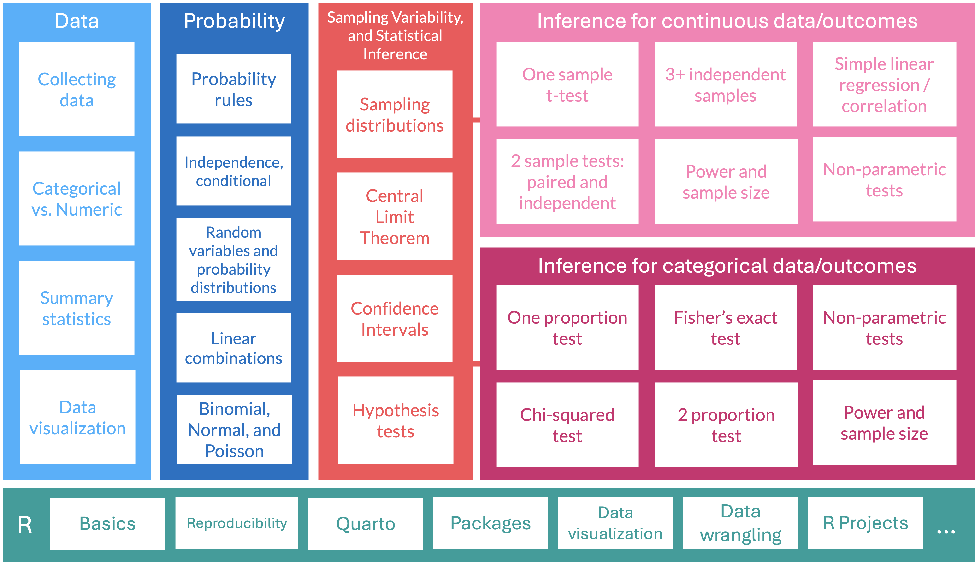
Where are we?

A little while ago…

We looked at inference for a single mean
We looked at inference for a difference in means from two independent samples

If there are two groups, we could see if they had different means by testing if the difference between the means were the same (null) or different (alternative)

What happens when we want to compare two or more groups’ means?
- Can no longer rely on the difference in means
- Need a new method to make inference (ANOVA or Linear Regression!)

Learning Objectives

Revisit data visualization for a numeric outcome and categorical variable (from Lesson 8).

Understand the different measures of variability within an Analysis of Variance (ANOVA) table.
Understand the F-statistic and F-distribution that is used to measure the ratio of between group and within group variability.
Determine if groups of means are different from one another using a hypothesis test and F-distribution.

From Lesson 8: Data visualization

Study investigating whether ACTN3 genotype at a particular location (residue 577) is associated with change in muscle function

Categorical variable: genotypes (CC, TT, CT)

Numeric variable: Muscle function, measured as percent change in non-dominant arm strength

We can start the investigation by plotting the relationship

From Lesson 8: Side-by-side boxplots with data points

We can look at the boxplot of percent change for each genotype with points shown so we can see the distribution of observations better

ggplot(data = famuss, 
       aes(x = actn3.r577x, 
           y = ndrm.ch)) + 
  geom_boxplot() + 
  labs(x = "ACTN3 genotype", 
       y = "Percent Change in Non-Dominant Arm Strength")  +
  geom_jitter(aes(color = actn3.r577x), 
    alpha = 0.3,      
    show.legend = FALSE,      
    position = position_jitter(     
      height = 0.4))

From Lesson 8: Ridgeline plot

Overlapped densities were easy enough to see with 3 genotypes
If you have many categories, a ridgeline plot might make it easier to see

library(ggridges)
ggplot(data = famuss, 
       aes(y = actn3.r577x, 
           x = ndrm.ch, 
           fill = actn3.r577x)) +
  geom_density_ridges(alpha = 0.3, 
          show.legend = FALSE) +      
  labs(x = "Percent Change in Non-Dominant Arm Strength",
       y = "ACTN3 genotype",
       title = "Strength change by genotype")

Poll Everywhere Question 1

Learning Objectives

Revisit data visualization for a numeric outcome and categorical variable (from Lesson 8).

Understand the different measures of variability within an Analysis of Variance (ANOVA) table.

Understand the F-statistic and F-distribution that is used to measure the ratio of between group and within group variability.
Determine if groups of means are different from one another using a hypothesis test and F-distribution.

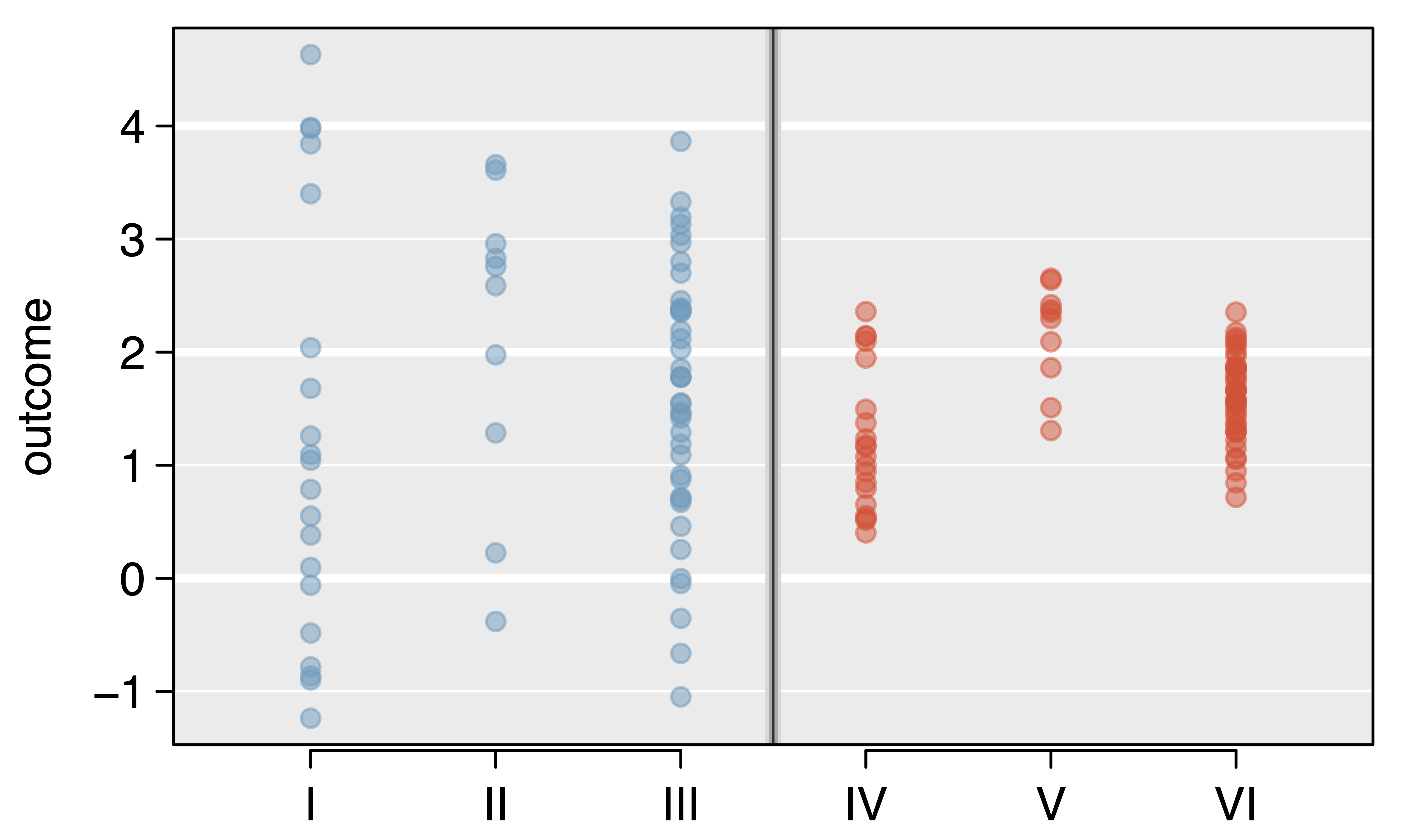
Comparing means

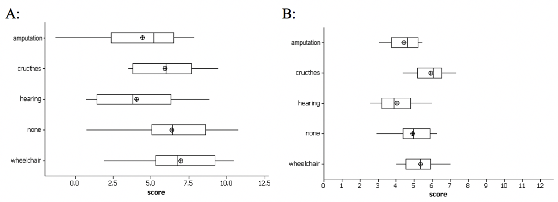
Whether or not two means are significantly different depends on:

How far apart the means are
How much variability there is within each group

Questions:

How to measure variability between groups?
How to measure variability within groups?
How to compare the two measures of variability?
How to determine significance?

Generic ANOVA table

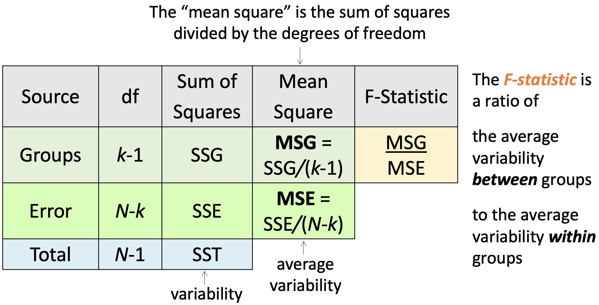
ANOVA: Analysis of Variance

ANOVA compares the variability between groups to the variability within groups

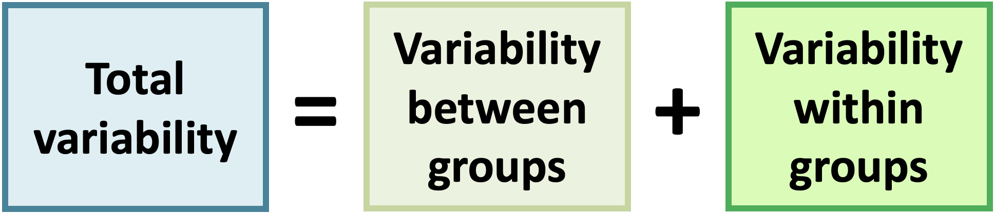
ANOVA: Analysis of Variance

Analysis of Variance (ANOVA) compares the variability between groups to the variability within groups

\[\sum_{i = 1}^k \sum_{j = 1}^{n_i}(x_{ij} -\bar{x})^2 \ \ = \ \sum_{i = 1}^k n_i(\bar{x}_{i}-\bar{x})^2 \ \ + \ \ \sum_{i = 1}^k\sum_{j = 1}^{n_i}(x_{ij}-\bar{x}_{i})^2\]

Notation

k groups
\(n_i\) observations in each of the k groups
Total sample size is \(N=\sum_{i=1}^{k}n_i\)
\(\bar{x}_{i}\) = mean of observations in group i
\(\bar{x}\) = mean of all observations
\(s_{i}\) = sd of observations in group i
\(s\) = sd of all observations

Observation	i = 1	i = 2	i = 3	\(\ldots\)	i = k	overall
j = 1	\(x_{11}\)	\(x_{21}\)	\(x_{31}\)	\(\ldots\)	\(x_{k1}\)
j = 2	\(x_{12}\)	\(x_{22}\)	\(x_{32}\)	\(\ldots\)	\(x_{k2}\)
j = 3	\(x_{13}\)	\(x_{23}\)	\(x_{33}\)	\(\ldots\)	\(x_{k3}\)
j = 4	\(x_{14}\)	\(x_{24}\)	\(x_{34}\)	\(\ldots\)	\(x_{k4}\)
\(\vdots\)	\(\vdots\)	\(\vdots\)	\(\vdots\)	\(\ddots\)	\(\vdots\)
j = \(n_i\)	\(x_{1n_1}\)	\(x_{2n_2}\)	\(x_{3n_3}\)	\(\ldots\)	\(x_{kn_k}\)
Means	\(\bar{x}_{1}\)	\(\bar{x}_{2}\)	\(\bar{x}_{3}\)	\(\ldots\)	\(\bar{x}_{k}\)	\(\bar{x}\)
Variance	\({s}^2_{1}\)	\({s}^2_{2}\)	\({s}^2_{3}\)	\(\ldots\)	\({s}^2_{k}\)	\({s}^2\)

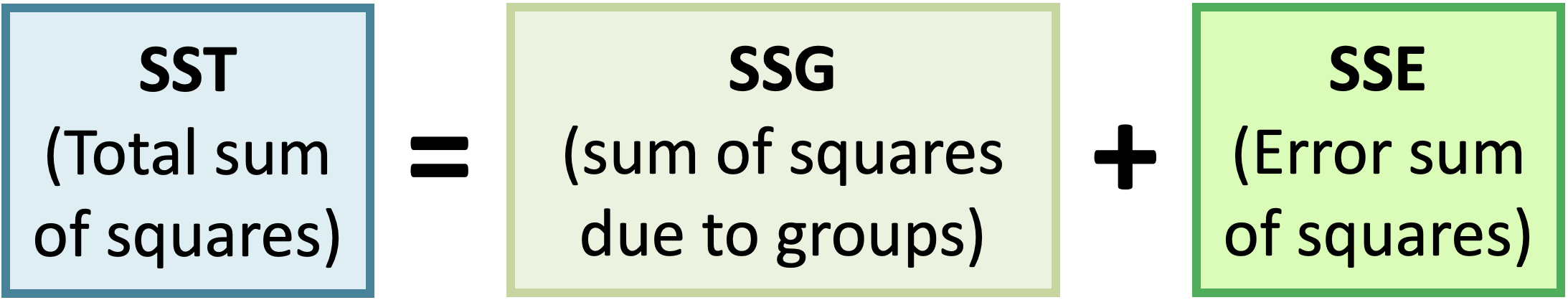
Total Sums of Squares (SST)

Total Sums of Squares:

\[SST = \sum_{i = 1}^k \sum_{j = 1}^{n_i}(x_{ij} -\bar{x})^2 = (N-1)s^2\]

where
- \(N=\sum_{i=1}^{k}n_i\) is the total sample size and
- \(s^2\) is the grand standard deviation of all the observations
This is the sum of the squared differences between each observed \(x_{ij}\) value and the grand mean, \(\bar{x}\).
That is, it is the total deviation of the \(x_{ij}\)’s from the grand mean.

Sums of Squares due to Groups (SSG)

Sums of Squares due to Groups:

\[SSG = \sum_{i = 1}^k n_i(\bar{x}_{i}-\bar{x})^2\]

This is the sum of the squared differences between each group mean, \(\bar{x}_{i}\), and the grand mean, \(\bar{x}\).
That is, it is the deviation of the group means from the grand mean.
Also called the Model SS, or \(SS_{model}.\)

Sums of Squares Error (SSE)

Sums of Squares Error:

\[SSE = \sum_{i = 1}^k\sum_{j = 1}^{n_i}(x_{ij}-\bar{x}_{i})^2 = \sum_{i = 1}^k(n_i-1)s_{i}^2\] where \(s_{i}\) is the standard deviation of the \(i^{th}\) group

This is the sum of the squared differences between each observed \(x_{ij}\) value and its group mean \(\bar{x}_{i}\).
That is, it is the deviation of the \(x_{ij}\)’s from the predicted ndrm.ch by group.
Also called the residual sums of squares, or \(SS_{residual}.\)

Poll Everywhere Question 2

ANOVA table to hypothesis test?

Okay, so how do we use all these types of variability to run a test?
How do we determine, statistically, if the groups have different means or not?

Answer: We use the F-statistic in a hypothesis test!

Learning Objectives

Revisit data visualization for a numeric outcome and categorical variable (from Lesson 8).
Understand the different measures of variability within an Analysis of Variance (ANOVA) table.

Understand the F-statistic and F-distribution that is used to measure the ratio of between group and within group variability.

Determine if groups of means are different from one another using a hypothesis test and F-distribution.

Thinking about the F-statistic

If the groups are actually different, then which of these is more accurate?

The variability between groups should be higher than the variability within groups
The variability within groups should be higher than the variability between groups

If there really is a difference between the groups, we would expect the F-statistic to be which of these:

Higher than we would observe by random chance
Lower than we would observe by random chance

The F-statistic

F-statistic represents the standardized ratio of variability between groups to the variability within the groups

\[F_{stat} = \dfrac{MSG}{MSE}\]

F is larger when the variability between groups is larger than variability within groups

The F-distribution

The F-distribution is skewed right
The F-distribution has two different degrees of freedom:
- one for the numerator of the ratio (k – 1) and
- one for the denominator (N – k)
\(p\)-value
- \(P(F > F_{stat})\)
- is always the upper tail
- (the area as extreme or more extreme)

Poll Everywhere Question 3

Learning Objectives

Revisit data visualization for a numeric outcome and categorical variable (from Lesson 8).
Understand the different measures of variability within an Analysis of Variance (ANOVA) table.
Understand the F-statistic and F-distribution that is used to measure the ratio of between group and within group variability.

Determine if groups of means are different from one another using a hypothesis test and F-distribution.

Reference: Steps in a Hypothesis Test

Check the assumptions
Set the level of significance \(\alpha\)
Specify the null ( \(H_0\) ) and alternative ( \(H_A\) ) hypotheses
1. In symbols
2. In words
3. ~~Alternative: one- or two-sided?~~
Calculate the test statistic.
Calculate the p-value based on the observed test statistic and its sampling distribution
Write a conclusion to the hypothesis test
1. Do we reject or fail to reject \(H_0\)?
2. Write a conclusion in the context of the problem

Step 1: Check assumptions

The sampling distribution is an F-distribution, if…

Sample sizes in each group group are large (each \(n \ge 30\))
- OR the data are relatively normally distributed in each group
Variability is “similar” in all group groups:
- Is the within group variability about the same for each group?
- As a rough rule of thumb, this condition is violated if the standard deviation of one group is more than double the standard deviation of another group

Step 1: Check assumptions

Use R to check both assumptions in our example

genotype_groups <- famuss %>% 
  group_by(actn3.r577x) %>% 
  summarise(count = n(), 
            SD = sd(ndrm.ch))
genotype_groups

# A tibble: 3 × 3
  actn3.r577x count    SD
  <fct>       <int> <dbl>
1 CC            173  30.0
2 CT            261  33.2
3 TT            161  35.7

Counts in each group are greater than 30!

max(genotype_groups$SD) / min(genotype_groups$SD)

[1] 1.191455

Variability in one group vs. another is no more than 1.2 times!

Step 3: Specify Hypotheses

General hypotheses

To test for a difference in means across k groups:

\[\begin{align} H_0 &: \mu_1 = \mu_2 = ... = \mu_k\\ \text{vs. } H_A&: \text{At least one pair } \mu_i \neq \mu_j \text{ for } i \neq j \end{align}\]

Hypotheses test for example

\[\begin{align} H_0 &: \mu_{CC} = \mu_{CT} = \mu_{TT}\\ \text{vs. } H_A&: \text{At least one pair } \mu_i \neq \mu_j \text{ for } i \neq j \end{align}\]

Step 4-5: Find the test statistic and p-value

Our test statistic is an F-statistic
- F-statistic: measurement of the ratio of variability between groups to variability within groups

Our F-statistic follows an F-distribution
- Which is why we cannot use something like the Z-distribution nor T-distribution

So we’ll need to find the F-statistic and its corresponding p-value using an F-distribution

Step 4-5: Find the test statistic and p-value

There are several options to run an ANOVA model (aka calculate F-statistic and p-value)
Two most common are lm and aov
- lm = linear model; will be using frequently in BSTA 512

lm(ndrm.ch ~ actn3.r577x, 
    data = famuss) %>% anova()

Analysis of Variance Table

Response: ndrm.ch
             Df Sum Sq Mean Sq F value  Pr(>F)  
actn3.r577x   2   7043  3521.6  3.2308 0.04022 *
Residuals   592 645293  1090.0                  
---
Signif. codes:  0 '***' 0.001 '**' 0.01 '*' 0.05 '.' 0.1 ' ' 1

aov(ndrm.ch ~ actn3.r577x, 
    data = famuss) %>% summary()

             Df Sum Sq Mean Sq F value Pr(>F)  
actn3.r577x   2   7043    3522   3.231 0.0402 *
Residuals   592 645293    1090                 
---
Signif. codes:  0 '***' 0.001 '**' 0.01 '*' 0.05 '.' 0.1 ' ' 1

Step 6: Conclusion

\[\begin{align} H_0 &: \mu_{CC} = \mu_{CT} = \mu_{TT}\\ \text{vs. } H_A&: \text{At least one pair} \mu_i \neq \mu_j \text{ for } i \neq j \end{align}\]

Recall the \(p\)-value = 0.0402
Use \(\alpha\) = 0.05
Do we reject or fail to reject \(H_0\)?

Conclusion statement:

There is sufficient evidence that at least one of the genotype groups has a change in arm strength statistically different from the other groups. ( \(p\)-value =0.0402)

Final note

Recall, visually the three looked pretty close
This is the case that I would also do some work to report the means and standard deviations of each genotype’s percent change in non-dominant arm strength.

famuss %>% 
  group_by(actn3.r577x) %>% 
  summarise(count = n(),
            mean = mean(ndrm.ch),
            SD = sd(ndrm.ch))

# A tibble: 3 × 4
  actn3.r577x count  mean    SD
  <fct>       <int> <dbl> <dbl>
1 CC            173  48.9  30.0
2 CT            261  53.2  33.2
3 TT            161  58.1  35.7

Revised conclusion statement:

For people with CC genotype then mean percent change in arm non-dominant arm strength was 48.9% (SD = 30%). For CT, mean percent change was 53.2% (SD = 33.2%). For TT, mean percent change was 58.1% (SD = 35.7%). There is sufficient evidence that at least one of the genotype groups has a change in arm strength statistically different from the other groups. ( \(p\)-value =0.0402)