R06: ggplot2, Part 1

Nicky Wakim

2024-10-21

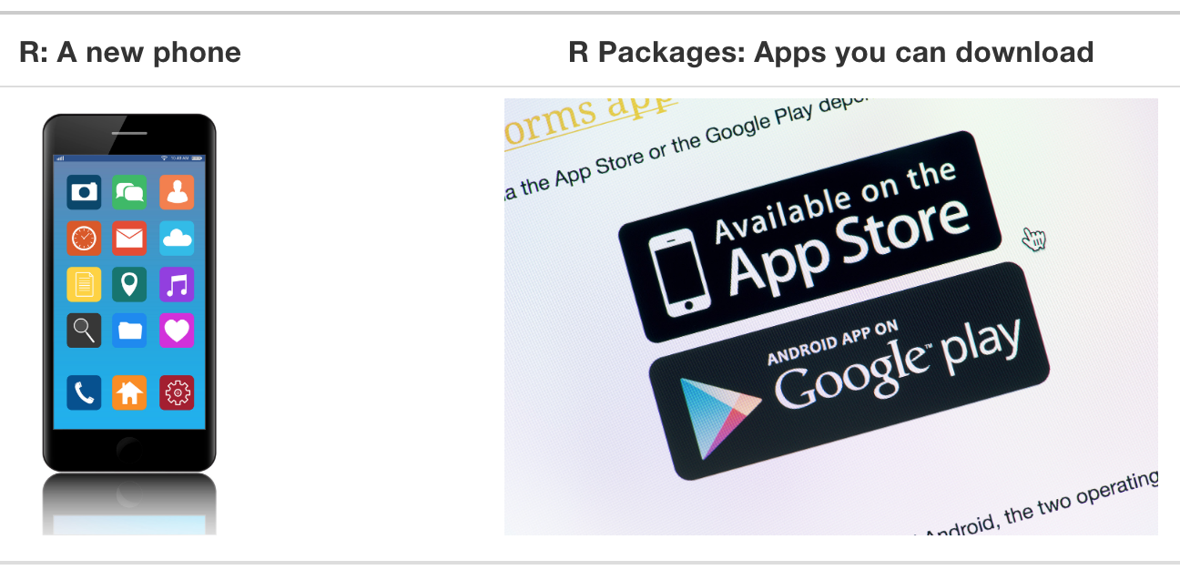
From last time: R Packages

A good analogy for R packages is that they are like apps you can download onto a mobile phone:

ModernDive Figure 1.4

From last time: Install the packages listed below

• knitr
  • this might actually already be installed
  • check your packages list
• tidyverse
  • this is actually a bundle of packages
  • Warning: it will take a while to install!!!
  • see more info at https://tidyverse.tidyverse.org/
• rstatix
  • for summary statistics of a dataset
• janitor
  • for cleaning and exploring data

• ggridges
  • for creating ridgeline plots
• devtools
  • used to create R packages
  • for our purposes, needed to install some packages
• oi_biostat_data
  • this package is on github
  • see the next slide for directions on how to install oi_biostat_data
• here
  • More info in slides ahead

From last time: Load packages with library() command

• Tip: at the top of your Qmd file, create a chunk that loads all of the R packages you want to use in that file.

• Use the library() command to load each required package.

  • Packages need to be reloaded every time you open Rstudio.
  • library() commands to load needed packages must be in the Qmd file

# run these every time you open Rstudio
library(tidyverse) # contains ggplot2    
library(oibiostat)
library(ggridges)
library(janitor)
library(rstatix)
library(knitr)
library(gtsummary) # NEW!!

• You can check whether a package has been loaded or not
  • by looking at the Packages tab and
  • seeing whether it has been checked off or not

Introduction to ggplot2

Artwork by @allison_horst

Artwork by @allison_horst

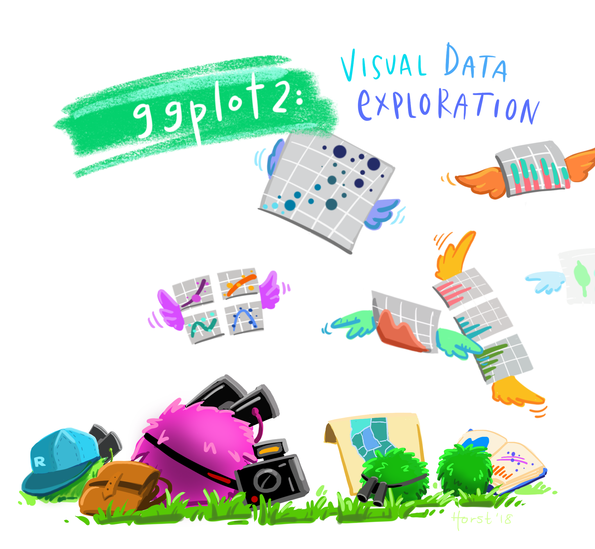
ggplot2 in tidyverse

• ggplot2 is tidyverse’s data visualization package

  • This is one of the main ways to create plots and explore data

 

• The gg in “ggplot2” stands for Grammar of Graphics

 

• It is inspired by the book Grammar of Graphics by Leland Wilkinson

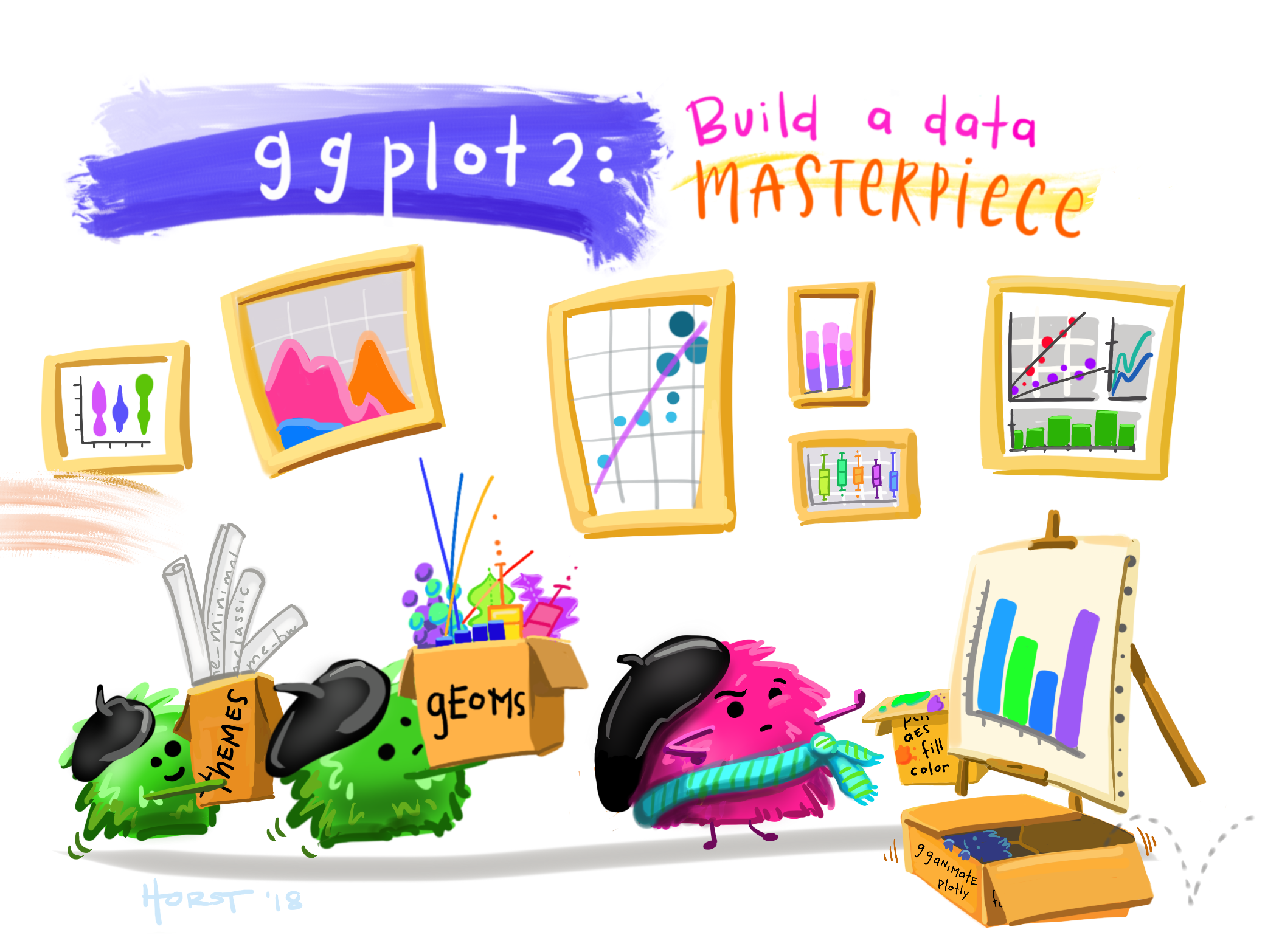
  • Make graphs/plots by combining independent components
  • Start with a basic plot then add layers

Works best with “tidy” data¹

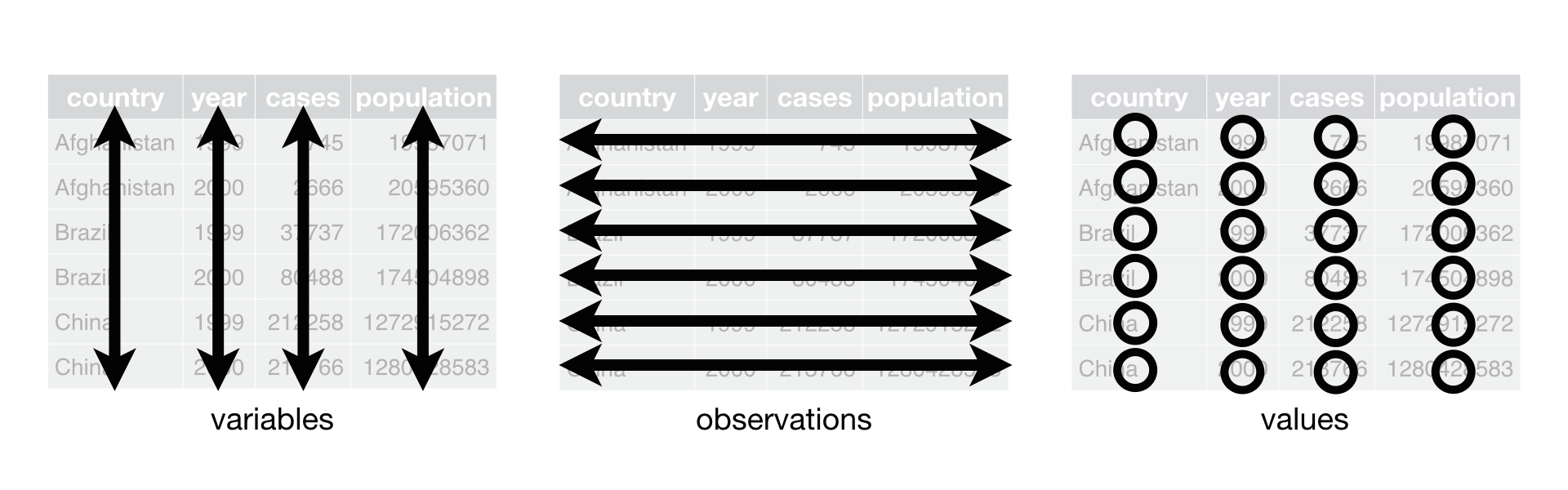
1. Each variable must have its own column.

2. Each observation must have its own row.

3. Each value must have its own cell.

1. Source: R for Data Science. Grolemund and Wickham.

Basics of a ggplot

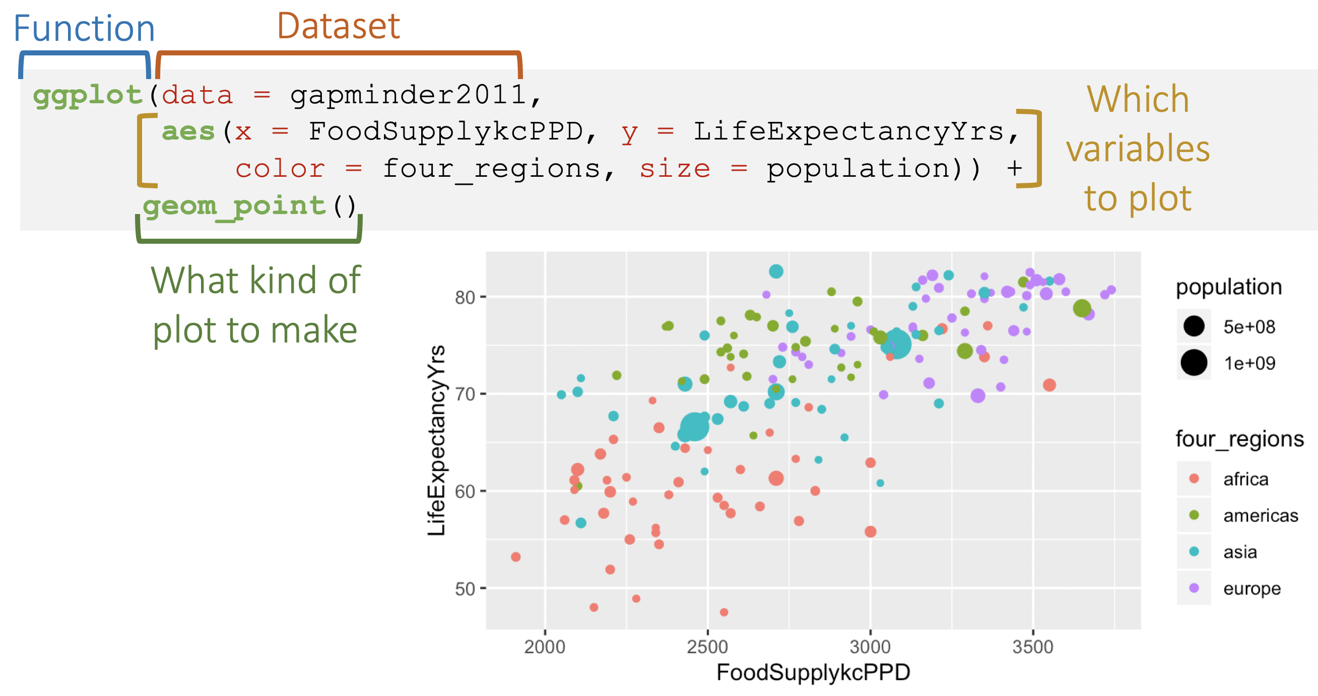
Grammar of ggplot2

• ggplot2 needs at least the following three to produce a chart:
  • data, a mapping, and a layer

 

• For the most part, there are default settings for the other parts:
  • scales, facets, coordinates, and themes

Data

• ggplot2 uses data to construct a plot

• Works best with tiday data (when every observation is a row and each variable is a column)

• First step in plotting:

  • Pass the data to the ggplot function, which stores the data to be used later by other parts of the plotting system

Data

• For example, if we intend to make a graphic about the mpg dataset, we would start as follows:

ggplot(data = mpg)

Mapping

• Mappings use the aes() function to map variables to the different axes on a plot

  • aes() stands for “aesthetics”

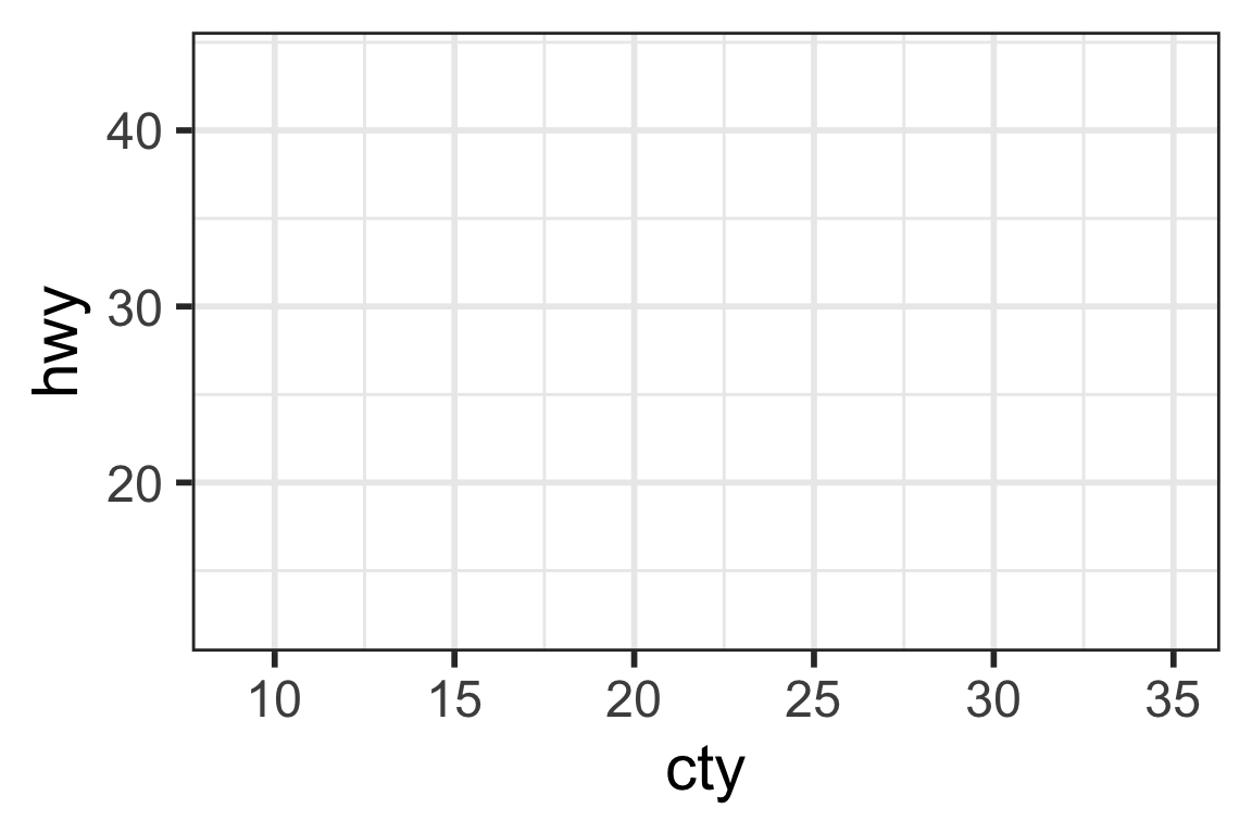
Data + Mapping

• If we want the cty and hwy columns to map to the x- and y-coordinates in the plot, we can do that as follows:

ggplot(mpg, mapping = aes(x = cty, y = hwy))

Layers

• Every layer consists of three important parts:

  • The geometry that determines how data are displayed, such as points, lines, or rectangles

  • The statistical transformation that may compute new variables from the data and affect what of the data is displayed.

  • The position adjustment that primarily determines where a piece of data is being displayed

• A layer can be constructed using the geom_*() and stat_*() functions

  • These functions often determine one of the three parts of a layer, while the other two can still be specified.

Data + Mapping + Layers

Here is how we can use two layers to display the cty and hwy columns of the mpg dataset as points and stack a trend line on top:

ggplot(mpg, aes(cty, hwy)) +
  # to create a scatterplot
  geom_point() +
  # to fit and overlay a line
  geom_smooth(formula = y ~ x, method = "lm")

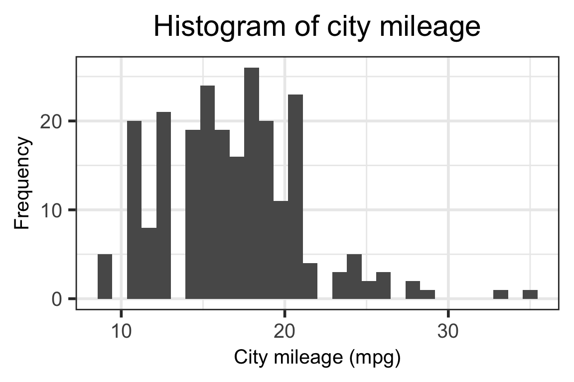
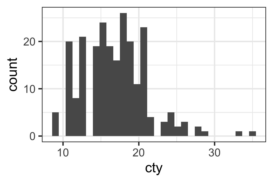
We can also make plots with a single variable

• Data: still mpg

• Mapping: using aesthetic to specify only one variable in the x-axis (cty)

• Layers: using geom_histogram() to show a plot of the counts per cty (which is city mileage)

ggplot(mpg, aes(cty)) +
  # to create a histogram
  geom_histogram()

Let’s take a second to try this out

• Make sure you are working in a Quarto document that has all the libraries loaded

• Use glimpse() to look at the variables in mpg

• Choose one of the variables to make a plot for

• Go to this site: https://bookdown.dongzhuoer.com/hadley/ggplot2-book/geom

  • Choose one of the “One variable” geoms that would work well for the variable you chose (discrete or continuous options)

• Make a plot for the variable!

05:00

We can add more to plots!

We can change labels!

ggplot(mpg, aes(cty)) +
  geom_histogram() +
  labs(x = "City mileage (mpg)", y = "Frequency", 
       title = "Histogram of city mileage")

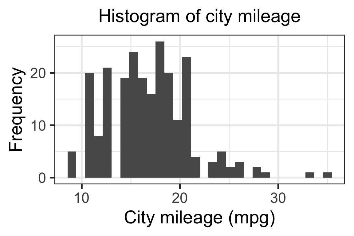
Adding more to plots!

Increase (or decrease) text size so we can read it / it fits nicely!

ggplot(mpg, aes(cty)) +
  geom_histogram() +
  labs(x = "City mileage (mpg)", y = "Frequency", 
       title = "Histogram of city mileage") +
  theme(axis.text = element_text(size = 15), 
        axis.title = element_text(size = 15), 
        title = element_text(size = 15))

Take a moment

• To add labels to your plot and change the text size if you want
• If you have time, look up help on the element_text() function
  • See if you can tilt your text or change the color

05:00

Resources on ggplot

• ggplot2 package website: https://ggplot2.tidyverse.org/articles/ggplot2.html
• Online textbook for ggplot2: https://ggplot2-book.org/
• Another online resource for data visualization with ggplot2: https://socviz.co/index.html#preface