R08: Transforming and subetting data with `tidyverse`

Nicky Wakim

2024-11-11

Introduction to the `tidyverse`

What is the tidyverse?

The tidyverse is a collection of R packages designed for data science. All packages share an underlying design philosophy, grammar, and data structures.

ggplot2 - data visualisation
dplyr - data manipulation
tidyr - tidy data
readr - read rectangular data
purrr - functional programming
tibble - modern data frames
stringr - string manipulation
forcats - factors
and many more …

Tidy data¹

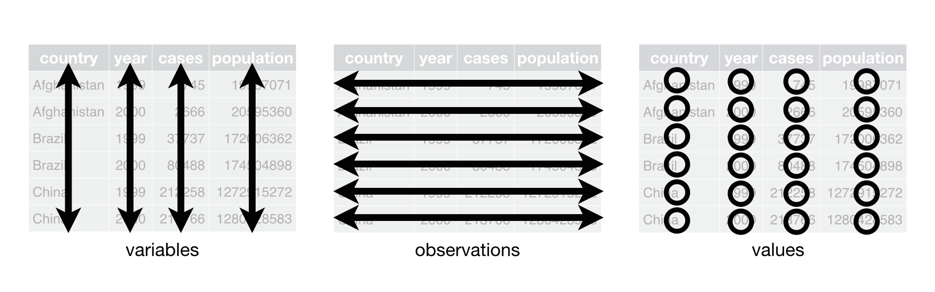
Each variable must have its own column.
Each observation must have its own row.
Each value must have its own cell.

Pipe operator (`magrittr`)

The pipe operator (%>%) allows us to step through sequential functions in the same way we follow if-then statements or steps from instructions

I want to find my keys, then start my car, then drive to work, then park my car.

Nested

park(drive(start_car(find("keys")), 
           to = "work"))

Piped

find("keys") %>%
  start_car() %>%
  drive(to = "work") %>%
  park()

Helpful functions for transforming and subsetting

Data transformation

rename()
mutate()
pivot_longer() and pivot_wider()

Data subsetting

filter()
select()

New dataset: `dds.discr`

In the US, individuals with developmental disabilities typically receive services and support from state governments
- California allocates funds to developmentally disabled residents through the Department of Developmental Services (DDS)
Dataset dds.discr
- Sample of 1,000 people who received DDS funds (out of a total of ~ 250,000)
- Data include age, sex, race/ethnicity, and annual DDS financial support per consumer

Let’s look back at the `dds.discr` dataset

We will load the data (This is a special case! dds.discr is a built-in R dataset)

data("dds.discr")

Now, let’s take a glimpse at the dataset:

glimpse(dds.discr)

Rows: 1,000
Columns: 6
$ id           <int> 10210, 10409, 10486, 10538, 10568, 10690, 10711, 10778, 1…
$ age.cohort   <fct> 13-17, 22-50, 0-5, 18-21, 13-17, 13-17, 13-17, 13-17, 13-…
$ age          <int> 17, 37, 3, 19, 13, 15, 13, 17, 14, 13, 13, 14, 15, 17, 20…
$ gender       <fct> Female, Male, Male, Female, Male, Female, Female, Male, F…
$ expenditures <int> 2113, 41924, 1454, 6400, 4412, 4566, 3915, 3873, 5021, 28…
$ ethnicity    <fct> White not Hispanic, White not Hispanic, Hispanic, Hispani…

Helpful functions for transforming and subsetting

Data transformation

rename()

mutate()
pivot_longer() and pivot_wider()

Data subsetting

filter()
select()

`rename()`: one of the first things I usually do

I notice that two variables have values that don’t necessarily match the variable name
- Female and male are not genders (NIH page on sex and gender)
- “White not Hispanic” combines race and ethnicity into one category (APA page on race and ethnicity)

I want to rename gender to sex (not sure if assigned at birth or current sex) and rename ethnicity to R_E (race and ethnicity)

`rename()`: one of the first things I usually do

rename() can change the name of a column
We use: data %>% rename(new_col_name = old_col_name)

dds.discr1 = dds.discr %>% 
  rename(SAB = gender, 
         R_E = ethnicity)

glimpse(dds.discr1)

Rows: 1,000
Columns: 6
$ id           <int> 10210, 10409, 10486, 10538, 10568, 10690, 10711, 10778, 1…
$ age.cohort   <fct> 13-17, 22-50, 0-5, 18-21, 13-17, 13-17, 13-17, 13-17, 13-…
$ age          <int> 17, 37, 3, 19, 13, 15, 13, 17, 14, 13, 13, 14, 15, 17, 20…
$ SAB          <fct> Female, Male, Male, Female, Male, Female, Female, Male, F…
$ expenditures <int> 2113, 41924, 1454, 6400, 4412, 4566, 3915, 3873, 5021, 28…
$ R_E          <fct> White not Hispanic, White not Hispanic, Hispanic, Hispani…

Helpful functions for transforming and subsetting

Data transformation

rename()

mutate()

pivot_longer() and pivot_wider()

Data subsetting

filter()
select()

`mutate()`: constructing new variables from what you have

We can create a new variable from other variables
- Another way to say it: creates new columns that are functions of existing variables
We often use it like:

data %>% mutate(new_variable = some_transformation_of_another_variable)

`mutate()`: create a new variable from two other variables

I want to make a variable that is the ratio of expenditures over age

dds.discr2 = dds.discr1 %>%
  mutate(exp_to_age = expenditures/age) 

glimpse(dds.discr2)

Rows: 1,000
Columns: 7
$ id           <int> 10210, 10409, 10486, 10538, 10568, 10690, 10711, 10778, 1…
$ age.cohort   <fct> 13-17, 22-50, 0-5, 18-21, 13-17, 13-17, 13-17, 13-17, 13-…
$ age          <int> 17, 37, 3, 19, 13, 15, 13, 17, 14, 13, 13, 14, 15, 17, 20…
$ SAB          <fct> Female, Male, Male, Female, Male, Female, Female, Male, F…
$ expenditures <int> 2113, 41924, 1454, 6400, 4412, 4566, 3915, 3873, 5021, 28…
$ R_E          <fct> White not Hispanic, White not Hispanic, Hispanic, Hispani…
$ exp_to_age   <dbl> 124.2941, 1133.0811, 484.6667, 336.8421, 339.3846, 304.40…

Recoding a numeric variable into categorical

Can we recreate age.cohort using the age varible?

summary(dds.discr2)

       id        age.cohort       age           SAB       expenditures  
 Min.   :10210   0-5  : 82   Min.   : 0.0   Female:503   Min.   :  222  
 1st Qu.:31809   6-12 :175   1st Qu.:12.0   Male  :497   1st Qu.: 2899  
 Median :55384   13-17:212   Median :18.0                Median : 7026  
 Mean   :54663   18-21:199   Mean   :22.8                Mean   :18066  
 3rd Qu.:76135   22-50:226   3rd Qu.:26.0                3rd Qu.:37713  
 Max.   :99898   51+  :106   Max.   :95.0                Max.   :75098  
                                                                        
                 R_E        exp_to_age    
 White not Hispanic:401   Min.   : 27.57  
 Hispanic          :376   1st Qu.:273.88  
 Asian             :129   Median :461.75  
 Black             : 59   Mean   :   Inf  
 Multi Race        : 26   3rd Qu.:938.12  
 American Indian   :  4   Max.   :   Inf  
 (Other)           :  5

Recoding a numeric variable into categorical (2/2)

We can integrate other functions into mutate()
For example, case_when() is a helpful function for mapping values to a category

Tidyverse:

dds.discr3 <- dds.discr2 %>%
  mutate(
    age.cohort2 = case_when(
          age <= 5 ~ "0-5",
          age <= 12 ~ "6-12", 
          age <= 17 ~ "13-17",
          age <= 21 ~ "18-21",
          age <= 50 ~ "22-50",
          age >= 51 ~ "51+"
    )
  )

Have you noticed that I change the number on `dds.discr`?

I change the number so that R saves a new dataset
And I do not overwrite the previous dataset
Can be annoying, but VERY helpful when you have to go back and change code
When you run things in real time and troubleshoot, it will be helpful to have different versions of the same dataframe

Helpful functions for transforming and subsetting

Data transformation

rename()
mutate()
pivot_longer() and pivot_wider()

Data subsetting

filter()

select()

`filter()`: keep rows that match a condition

What if I want to subset the data frame? (keep certain rows of observations)

I want to look at the data for people who between 50 and 60 years old

dds.discr4 = dds.discr3 %>%
  filter(age >= 50 & age <= 60)

glimpse(dds.discr4)

Rows: 23
Columns: 8
$ id           <int> 15970, 19412, 29506, 31658, 36123, 39287, 39672, 43455, 4…
$ age.cohort   <fct> 51+, 51+, 51+, 51+, 51+, 51+, 51+, 51+, 51+, 51+, 51+, 51…
$ age          <int> 51, 60, 56, 60, 59, 59, 54, 57, 52, 57, 55, 52, 59, 54, 5…
$ SAB          <fct> Female, Female, Female, Female, Male, Female, Female, Mal…
$ expenditures <int> 54267, 57702, 48215, 46873, 42739, 44734, 52833, 48363, 5…
$ R_E          <fct> White not Hispanic, White not Hispanic, White not Hispani…
$ exp_to_age   <dbl> 1064.0588, 961.7000, 860.9821, 781.2167, 724.3898, 758.20…
$ age.cohort2  <chr> "51+", "51+", "51+", "51+", "51+", "51+", "51+", "51+", "…

Helpful functions for transforming and subsetting

Data transformation

rename()
mutate()
pivot_longer() and pivot_wider()

Data subsetting

filter()

select()

`select()`: keep or drop columns using their names and types

What if I want to remove or keep certain variables?

I want to only have age and expenditure in my data frame

dds.discr5 = dds.discr2 %>%
  select(age, expenditures)

glimpse(dds.discr5)

Rows: 1,000
Columns: 2
$ age          <int> 17, 37, 3, 19, 13, 15, 13, 17, 14, 13, 13, 14, 15, 17, 20…
$ expenditures <int> 2113, 41924, 1454, 6400, 4412, 4566, 3915, 3873, 5021, 28…

Resources

`dplyr` resources

More dpylr functions to reference!

Additional details and examples are available in the vignettes:

and the dplyr 1.0.0 release blog posts:

R programming class at OHSU!

You can check out Dr. Jessica Minnier’s R class page if you want more notes, videos, etc.

The larger tidy ecosystem

Just to name a few…

Credit to Mine Çetinkaya-Rundel

These notes were built from Mine’s notes
- Most pages and code were left as she made them
- I changed a few things to match our class
Please see her Github repository for the original notes

If time

Tidy data¹

Each variable must have its own column.
Each observation must have its own row.
Each value must have its own cell.

How do we make our data tidy??

From a contingency table, we need to create the dataframe using the counts

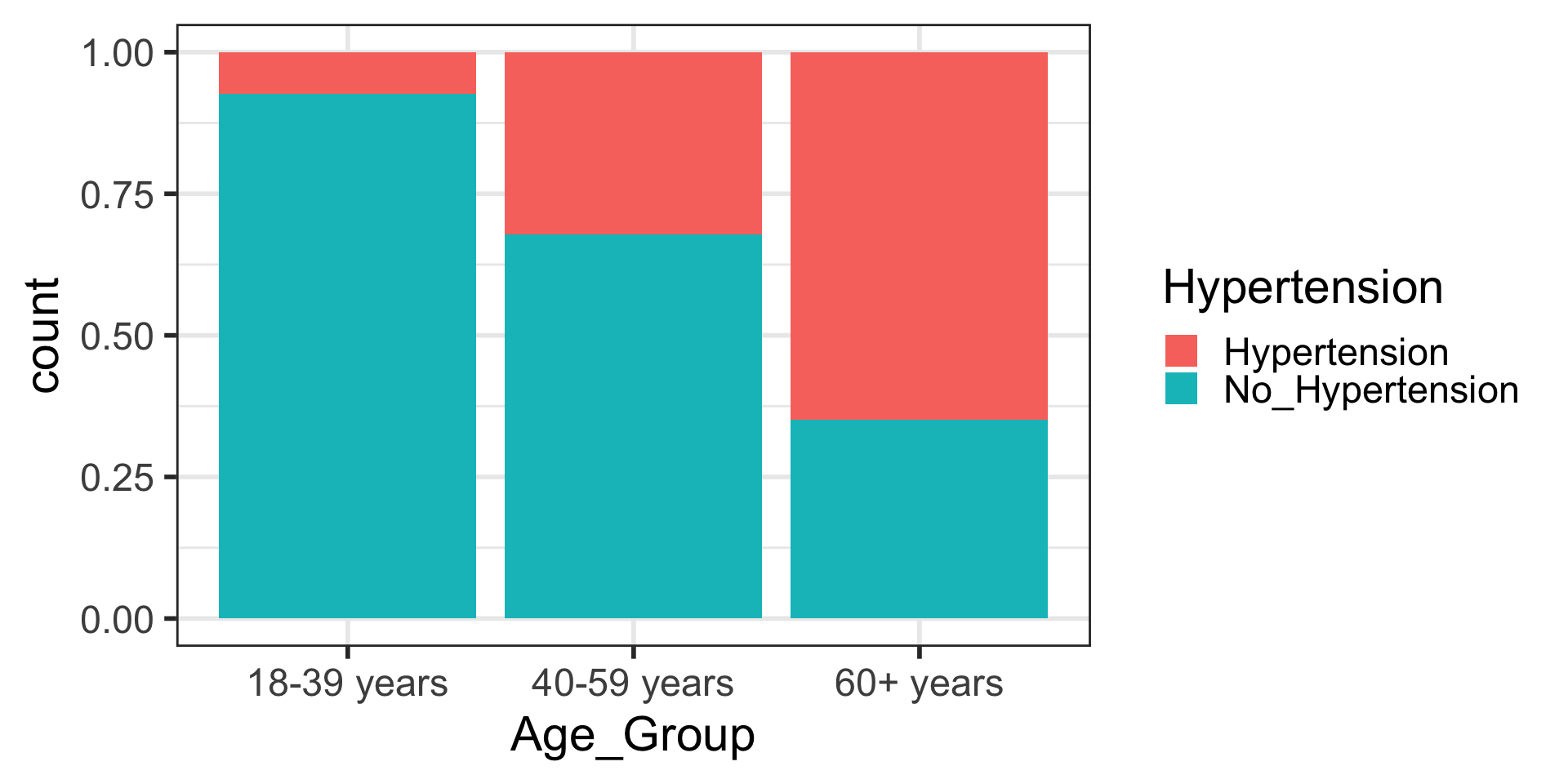
In Lesson 4, we saw this contingency table:

Table: Contingency table showing hypertension status and age group, in thousands.
Age Group	Hypertension	No Hypertension
18-39 yrs	8836	112206
40-59 yrs	42109	88663
60+ yrs	39917	21589

And then I magically had it in a new format so I could make this plot:

Code

ggplot(data = hyp_data, 
       aes(x = Age_Group, 
       fill = Hypertension)) + 
  geom_bar(position = "fill")

`pivot_*()` functions

I used `pivot_longer()` to create tidy data (1/2)

Note that you won’t be required to use pivot_longer()
- I will give you data in a tidy form
Here’s the original data frame:

hyp_cont <- data.frame(
  Age_Group = c("18-39 years", "40-59 years", "60+ years"),
  Hypertension = c(8836, 42109, 39917),
  No_Hypertension = c(112206, 88663, 21589) )

Note that I use use data.frame() to make a data frame
Then I can name each column that we saw in the contingency table
Note that information about hypertension vs no hypertension is split between columns
- And that we only have 3 rows of data to show all 313320 observations

I used `pivot_longer()` to create tidy data (2/2)

We need to tell pivot_longer():

Which column must be repeated (pivoted) (all other columns are not repeating)
The name of the new column that will contain the old variable names
Where the values in each cell under the old variables will go

hyp_data1 = pivot_longer(
              data = hyp_cont, 
              cols = -Age_Group,         # columns to pivot
              names_to = "Hypertension", # name of new column for variable names
              values_to = "Counts")     # name of new column for values
hyp_data1

# A tibble: 6 × 3
  Age_Group   Hypertension    Counts
  <chr>       <chr>            <dbl>
1 18-39 years Hypertension      8836
2 18-39 years No_Hypertension 112206
3 40-59 years Hypertension     42109
4 40-59 years No_Hypertension  88663
5 60+ years   Hypertension     39917
6 60+ years   No_Hypertension  21589

One more step to make it tidy

Aka we need one more step to make it so every row is an observation
- In this case, we want each row to represent data from one person

hyp_data = hyp_data1 %>% uncount(Counts)
head(hyp_data, 10)

# A tibble: 10 × 2
   Age_Group   Hypertension
   <chr>       <chr>       
 1 18-39 years Hypertension
 2 18-39 years Hypertension
 3 18-39 years Hypertension
 4 18-39 years Hypertension
 5 18-39 years Hypertension
 6 18-39 years Hypertension
 7 18-39 years Hypertension
 8 18-39 years Hypertension
 9 18-39 years Hypertension
10 18-39 years Hypertension

R08: Transforming and subetting data with tidyverse

Introduction to the tidyverse

What is the tidyverse?

Tidy data1

Pipe operator (magrittr)

Helpful functions for transforming and subsetting

Helpful functions for transforming and subsetting

New dataset: dds.discr

Let’s look back at the dds.discr dataset

Helpful functions for transforming and subsetting

rename(): one of the first things I usually do

rename(): one of the first things I usually do

Helpful functions for transforming and subsetting

mutate(): constructing new variables from what you have

mutate(): create a new variable from two other variables

Recoding a numeric variable into categorical

Recoding a numeric variable into categorical (2/2)

Have you noticed that I change the number on dds.discr?

Helpful functions for transforming and subsetting

filter(): keep rows that match a condition

Helpful functions for transforming and subsetting

select(): keep or drop columns using their names and types

Resources

dplyr resources

R programming class at OHSU!

The larger tidy ecosystem

Credit to Mine Çetinkaya-Rundel

If time

Tidy data1

How do we make our data tidy??

pivot_*() functions

I used pivot_longer() to create tidy data (1/2)

I used pivot_longer() to create tidy data (2/2)

One more step to make it tidy

R08: Transforming and subetting data with `tidyverse`

Introduction to the `tidyverse`

Tidy data¹

Pipe operator (`magrittr`)

New dataset: `dds.discr`

Let’s look back at the `dds.discr` dataset

`rename()`: one of the first things I usually do

`rename()`: one of the first things I usually do

`mutate()`: constructing new variables from what you have

`mutate()`: create a new variable from two other variables

Have you noticed that I change the number on `dds.discr`?

`filter()`: keep rows that match a condition

`select()`: keep or drop columns using their names and types

`dplyr` resources

Tidy data¹

`pivot_*()` functions

I used `pivot_longer()` to create tidy data (1/2)

I used `pivot_longer()` to create tidy data (2/2)