Outcomes, Events, and Sample Space
Note that I will keep the example and definition numbering that is presented in the textbook, so it may seem like numbers are being skipped. This just means I may not have presented an example from the textbook here. Feel free to consult the textbook for more examples!
1.1 Introduction
The introduction in this chapter starts with the following quote:
I couldn’t say it better myself. There are examples with obvious hints at randomness (i.e. dice rolls, coins flips) and there are examples with not-so-obvious randomness involved (i.e. time until any given traffic light turns green).
Our goal in probability and statistics is to characterize randomness. Then as statisticians, we can use what we know about randomness to see if certain features of the world is within randomness or outside the randomness. For example, according to a New York Times article published on July 25, 2023, the Education Department is investigating Harvard University’s legacy admissions policy. Here is an excerpt from that article:
Harvard gives preference to applicants who are recruited athletes, legacies, relatives of donors and children of faculty and staff. As a group, they make up less than 5 percent of applicants, but around 30 percent of those admitted each year. About 67.8 percent of these applicants are white, according to court papers.
Using probability, we can start to see why this practice might be inequitable. If these applicants make up 5% of the total applicant pool, and we completely, randomly chose applicants to admit, then we would expect 5% of admitted students to be this group of recruited athletes, legacies, relatives of donors, and children of faculty and staff. We could argue that recruited athletes are more likely to be admitted since they are, in fact, recruited, or that children of faculty and staff might “game” high school succesfully because they live in a home that subscribes to the academic world. If we want to compare the acceptance rate of 30% for this group to the average acceptance rate, the article actually fails to present a crucial peice of information: the average acceptance rate. I looked it up, and it is ~4%. So now we can start to think about questions like: With an average acceptance rate of 4%, does an acceptance of 30% of this group of recruited athletes, legacies, relatives of donors and children of faculty and staff make sense? We will explore this example further as we progress through our class.
Baaack to our definitions: When we have several potential outcomes, and an event is a collection of outcomes, then we can start thinking of the set of potential outcomes. When there are no outcomes, then we have the empty set \(\emptyset\). When we look at all outcomes, we call it the sample space \(S\). For now, when we look at a single event, we will focus on the sample space. When we start thinking of multiple events, the empty set might come into play. And just to reiterate: The empty set is an event. It is an impossible event, but it is still considered an event. So when you consider all possible events, the empty set is included. When you consider all possible outcomes, this is the sample space.
Now let’s look at at an example with an obvious hint at randomness:
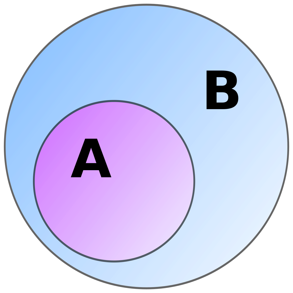
We introduced subset, but here’s the definition:
Event A is a subset of event B, written \(A \subset B\). if every outcome in A is also an outcome in B.
Let’s work on defining different types of events within sample spaces:
Definitions:
1.2 Complements and DeMorgan’s Laws
Notes
There are a few things I’d like to address from the book:
There is a set of examples, 1.5 and 1.6, that talk about the birth of a baby. While this example is helpful for considering potential sample spaces, there is an oversight on the biology of births. The examples refer to the event of the sex assigned at birth (SAB). There are two issues in this example. First, SAB is considered binary in this example (I will get back to this). Second, the binary SAB is written as “boy” or “girl.” These labels have gender identity inherently attached to their meaning, and thus, the more accurate binary versions of these are “male” or “female,” respectively (“Assigned Sex at Birth,” n.d.). These are often denoted as “assigned male at birth” (AMAB) or “assigned female at birth” (AFAB). Going back the first issue, a binary representation of SAB does not cover all possible events. People can also be intersex, meaning their genitals, chromosomes, and/or reproductive organs are not exclusively AMAB or AFAB (“Intersex: What Is Intersex, Gender Identity, Intersex Surgery,” n.d.).