(polygon[GRID.polygon.1], polygon[GRID.polygon.2], polygon[GRID.polygon.3], polygon[GRID.polygon.4], text[GRID.text.5], text[GRID.text.6], text[GRID.text.7], text[GRID.text.8], text[GRID.text.9]) EPI 525
These are the some numeric/short answers to the homework. Often, these answers are insufficient for your own work or solutions. I just wanted to give you a part of the answer to help guide you in the right direction.
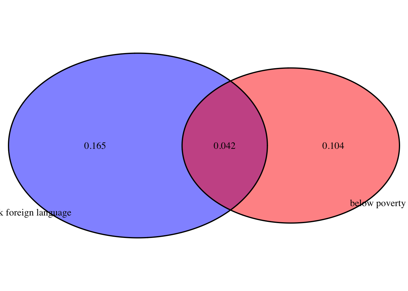
The American Community Survey is an ongoing survey that provides data every year to give communities the current information they need to plan investments and services. The 2010 American Community Survey estimates that 14.6% of Americans live below the poverty line, 20.7% speak a language other than English (foreign language) at home, and 4.2% fall into both categories.
Not disjoint
(polygon[GRID.polygon.1], polygon[GRID.polygon.2], polygon[GRID.polygon.3], polygon[GRID.polygon.4], text[GRID.text.5], text[GRID.text.6], text[GRID.text.7], text[GRID.text.8], text[GRID.text.9]) 10.4%
31.1%
68.9%
Not independent
0.32
0.57
0.68
0.1024
0.4624
| health_status | Excellent | Very_good | Good | Fair | Poor | Total |
|---|---|---|---|---|---|---|
| No | 459 | 727 | 854 | 385 | 99 | 2524 |
| Yes | 4198 | 6245 | 4821 | 1634 | 578 | 17476 |
| total | 4657 | 6972 | 5675 | 2019 | 677 | 20000 |
0.02295
0.3361
The Behavioral Risk Factor Surveillance System (BRFSS) is an annual telephone survey designed to identify risk factors in the adult population and report emerging health trends. The following table displays the distribution of health status of respondents to this survey (excellent, very good, good, fair, poor) conditional on whether or not they have health insurance.
(covg.tab <- data.frame(
  health_status = c("No","Yes","total"),
  Excellent = c(0.0230, 0.2099,0.2329),
  Very_good = c(0.0364, 0.3123,0.3486),
  Good = c(0.0427,0.2410,0.2838),
  Fair = c(0.0192,0.0817,0.1009),
  Poor = c(0.0050,0.0289,0.0338),
  Total = c(0.1262,0.8738,1.0000)
)) %>% gt()| health_status | Excellent | Very_good | Good | Fair | Poor | Total |
|---|---|---|---|---|---|---|
| No | 0.0230 | 0.0364 | 0.0427 | 0.0192 | 0.0050 | 0.1262 |
| Yes | 0.2099 | 0.3123 | 0.2410 | 0.0817 | 0.0289 | 0.8738 |
| total | 0.2329 | 0.3486 | 0.2838 | 0.1009 | 0.0338 | 1.0000 |
No
0.2329
0.2402152
0.1822504
No
0.605
0.9997
| age_group | prevalence | PPV |
|---|---|---|
| 30 - 40 | 0.0044 | 0.070 |
| 40 - 50 | 0.0147 | 0.202 |
| 50 - 60 | 0.0238 | 0.293 |
| 60 - 70 | 0.0356 | 0.386 |
| 70 - 80 | 0.0382 | 0.403 |
The PPV increased more with the higher specificity vs. the higher sensitivity.
0.05