1. Application of expected values and variance for discrete RVs
Expected value (mean) and variance, as we saw in this lesson about random variables, is the same as what we saw in Lesson 2 on numeric summaries! These are really good tools to calculate the center and spread of a distribution. In the case of a random variable with a Binomial distribution, this will tell us the expected number of “successes” and how spread out the number of successes are.
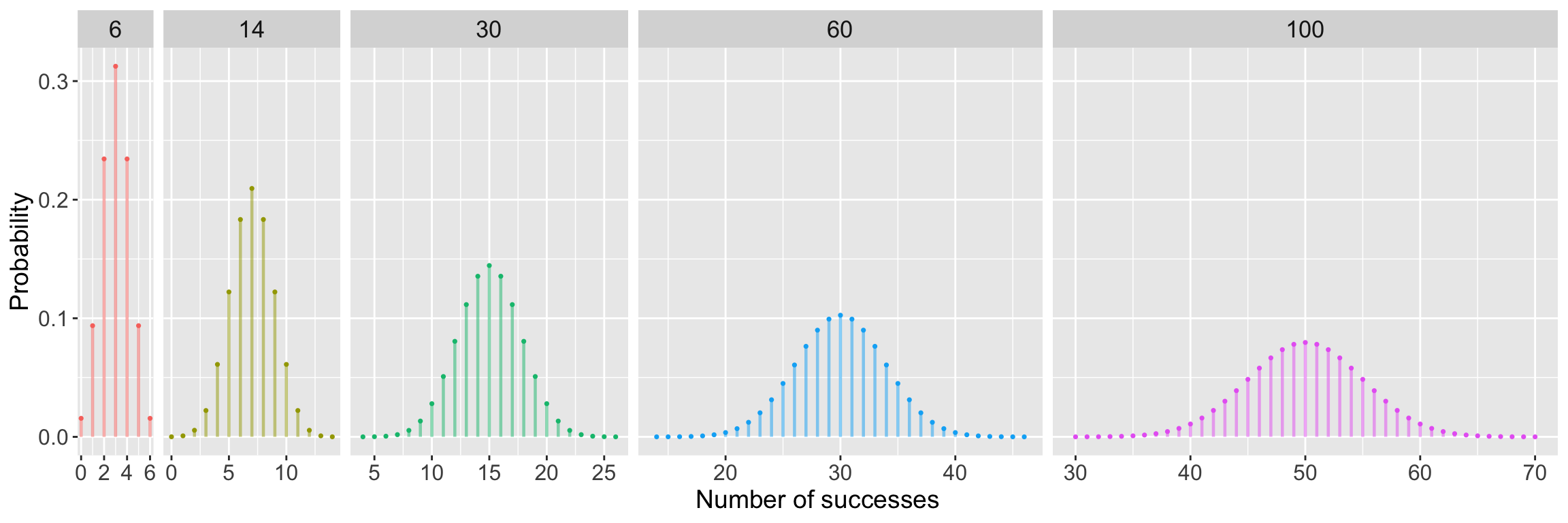
Let’s use some simulations to show this! The probability of success for all of these random variables is 0.5. The top part of the graphs shows \(n\), the number of trials. The centers and spreads for each of these random variables (all Binomally distributed) are different!
Code that I used to create these plots of binomial RVs
library(tidyverse)x <--5:250n =c(6,14,30,60,100)p =0.5binom =data.frame(x=rep(x, length(n)), y=dbinom(x, rep(n, each=length(x)), p),n=rep(n, each=length(x)))ggplot(binom %>%filter(y >1e-5) %>%group_by(n), aes(x, y, colour=factor(n))) +geom_point(size=0.6) +geom_segment(aes(x=x, xend=x, y=0, yend=y, colour=factor(n)), lwd=0.8, alpha=0.5) +facet_grid(. ~ n, scales="free", space="free") +theme(legend.position ="none",axis.title =element_text(size =14), # Axis title sizeaxis.text =element_text(size =12), # Axis text sizestrip.text =element_text(size =13)) +# Facet label sizelabs(x ="Number of successes", y ="Probability")
2. Use of these distributions
When it comes to important distributions in statistics, we want to get familiar with the the characteristics and calculations because it is an important step in the data analysis process.
Here is the basic data analysis process:
Recognize type of data we’re dealing with (continuous, discrete, categorical, ordinal, count?)
Determine the key characteristics of the data. What is it measuring? For example, count data can be out of a certain number of trials (binomial) or has no limit to the count (Poisson)
Identify the distribution of the data so we can easily describe/summarize the data (using known properties of the distribution)
Use specific tools that are designed specifically for that distribution to analyze the data (aka answer a specific research question)
3. Binomial distribution
Eek! I’ve ran out of time to organize and really get into this explanation. Instead, I’m going to drop a few links below. Keep Googling for other videos on Bernoulli and Binomial distributions! There are a lot out there, so let me know if one really resonates with you.
I wouldn’t get too caught up in the formula here. The important part of variance is that we measure the spread (as seen in Muddy Point 1) of a distribution or data.