Quarto and .qmd’s
What is Quarto?
- Quarto is a publishing system that lets us combine text and code into a single document
- It is the successor to R Markdown — you may see both names online, but we’ll use Quarto
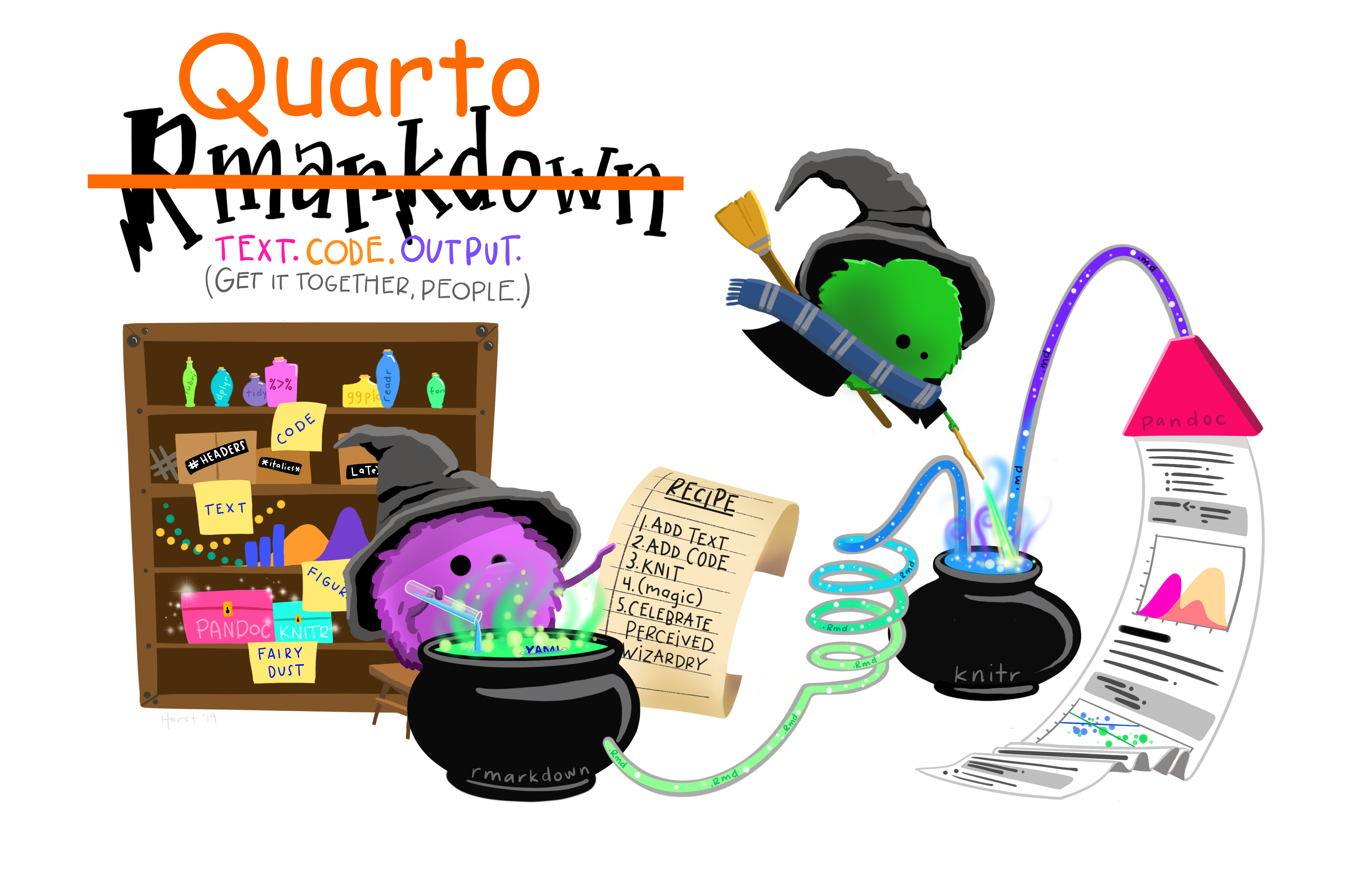
Artwork by @allison_horst
.qmd file = code + text
A .qmd file holds two things together:
- Code (R or other languages) — the same code you’d write in a script
- Text (like you’d write in Word) — headings, explanations, formatting
When you render the file, Quarto combines them into a polished output: .html, .pdf, .docx, and more.
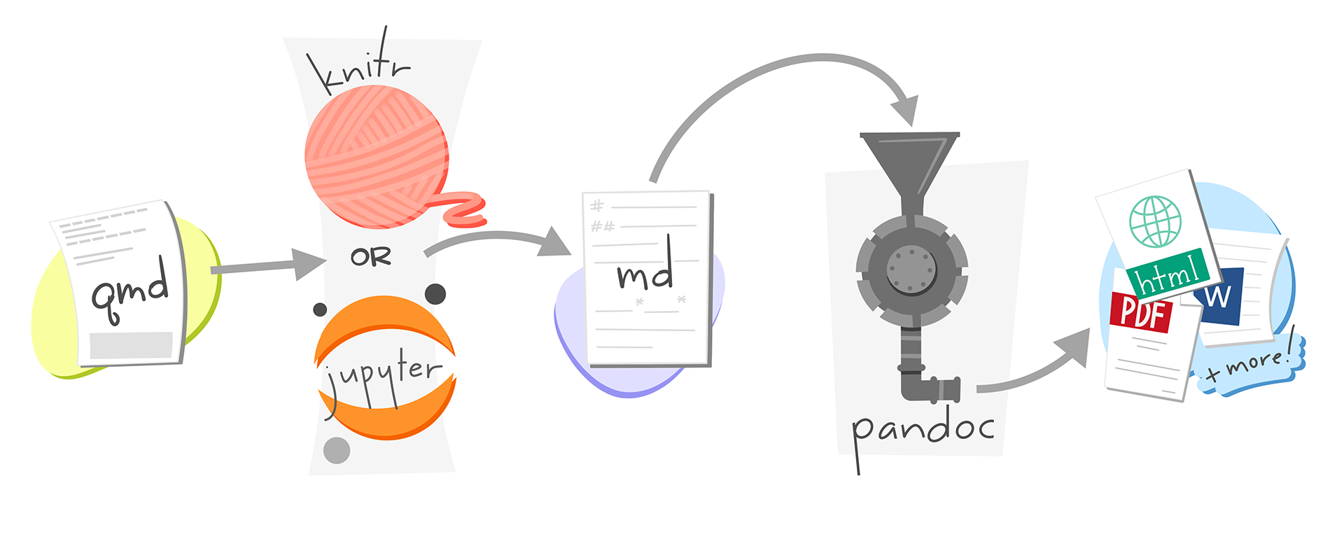
3 types of content in a .qmd
Every .qmd file is made up of exactly three things:
- YAML metadata — settings at the top of the file (title, author, output format)
- Text — plain writing, lists, images, links
- Code chunks — blocks of R (or other) code
We’ll look at each one in detail — but first, let’s see them all together in a real example.

3. Code chunks
Code chunks are where your R code lives
- There are 3 options to insert a new code chunk:
- Click the
![]() button at the top of the editor
button at the top of the editor - Keyboard shortcut: Command + Option + I (Mac) / Ctrl + Alt + I (PC)
- Type out
```{r}to start and```to close
 button at the top of the editor
Step 1: Create a Quarto file
Two options:
File→New File→Quarto Document...→OK- Click
![]() in the upper left →
in the upper left → ![]()
 in the upper left →
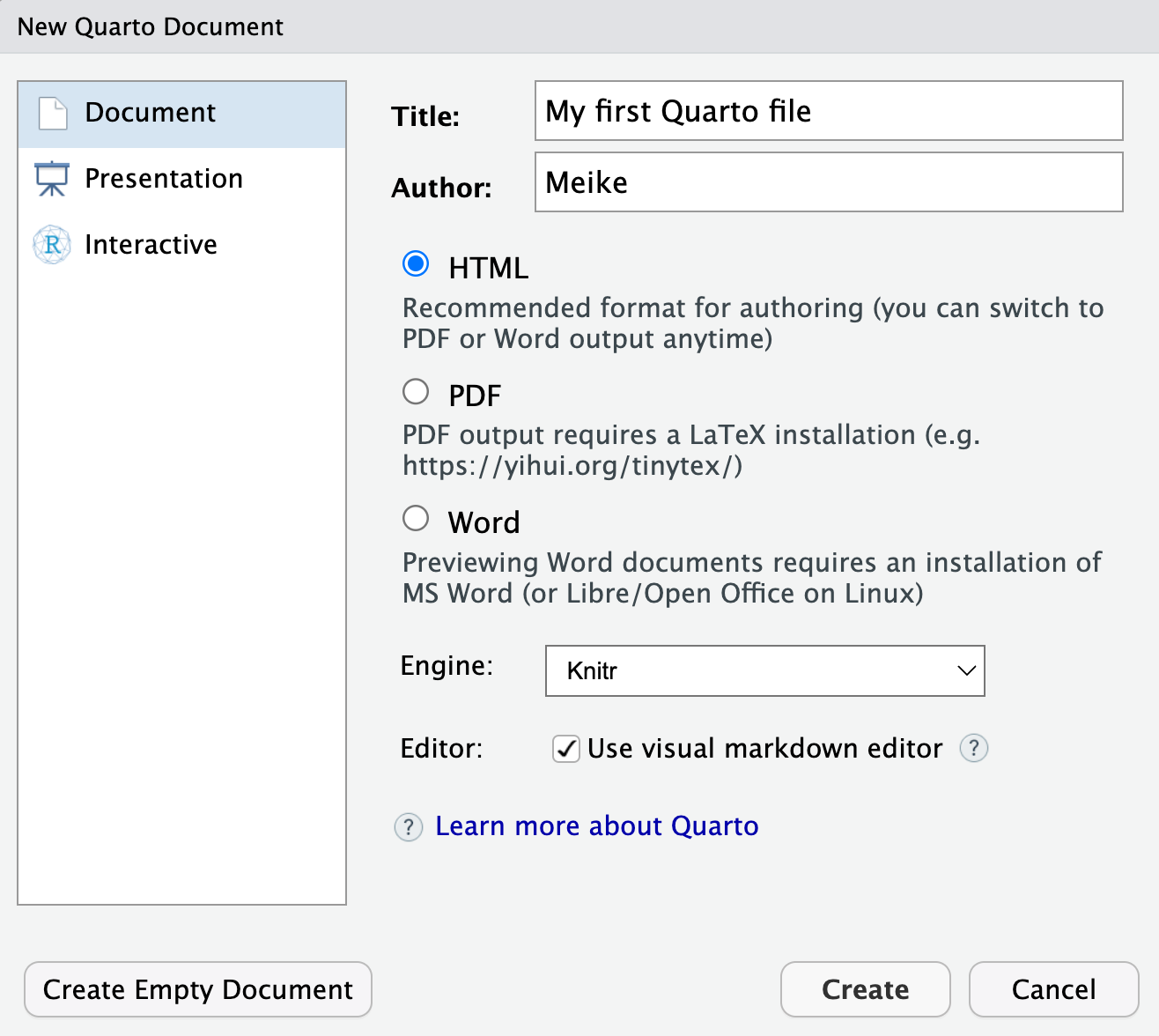
In the pop-up window:
- Enter a title and your name
- Output format:
HTML - Engine:
Knitr - Editor:
Use visual markdown editor - Click
Create
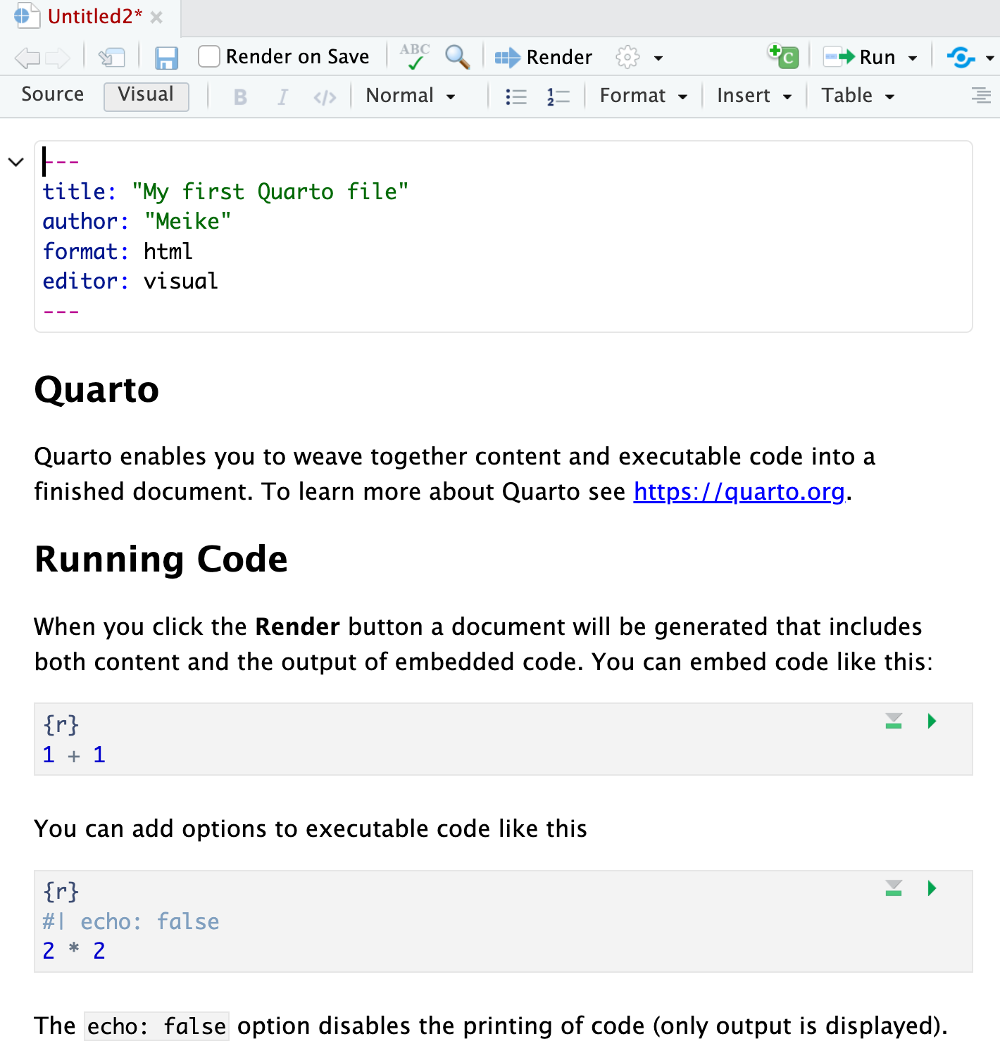
Step 2: Edit the file
- After clicking
Create, a template.qmdopens in your editor - Try editing the title in the YAML, or changing the text below it
- Make sure you only edit content at and below the
---that ends the YAML
Step 3: Save the file
File→Save- Click
![]() above the editor window
above the editor window - Keyboard shortcut: Ctrl + S (PC) / Command + S (Mac)
 above the editor window
When saving, specify:
- Filename — always use
.qmdas the extension - Folder — save under your lessons folder as
lesson#_quarto_work.qmd
Step 4: Render to HTML
Rendering turns your .qmd into a viewable .html file.
Two options:
- Click the Render icon
![]() at the top of the editor
at the top of the editor - Keyboard shortcut: Command + Shift + K (Mac) / Ctrl + Shift + K (PC)
 at the top of the editor
After rendering:
- A new window opens with the HTML output
- Both
.qmdand.htmlfiles appear in your folder — the HTML takes its name from the.qmd
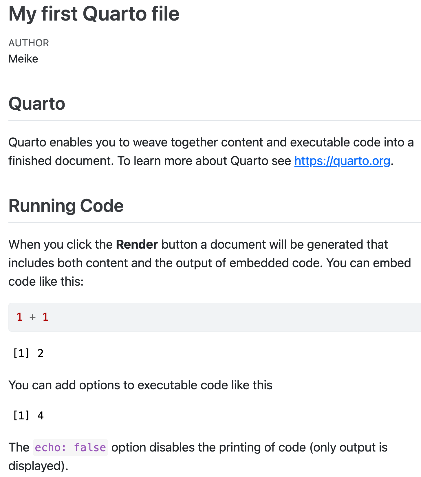
.qmd vs. .html output
- In this class, you’ll turn in both files
- Collaborators typically only need the
.html— they can view results without running any code themselves
.qmd file
.html output
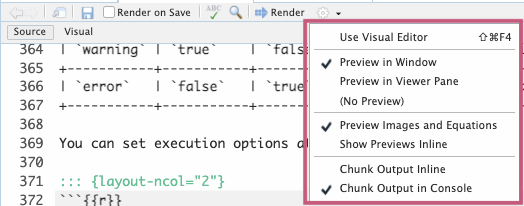
Tips: Customizing your setup
Where does the HTML preview open?
Preview in Window— opens in a browser tabPreview in Viewer Pane— opens in the bottom-right RStudio pane
Where does code output appear?
Chunk Output Inline— output appears below the chunk in the editorChunk Output in Console— output appears in the Console pane