Tidy data

Nicky Wakim

Tidy data¹

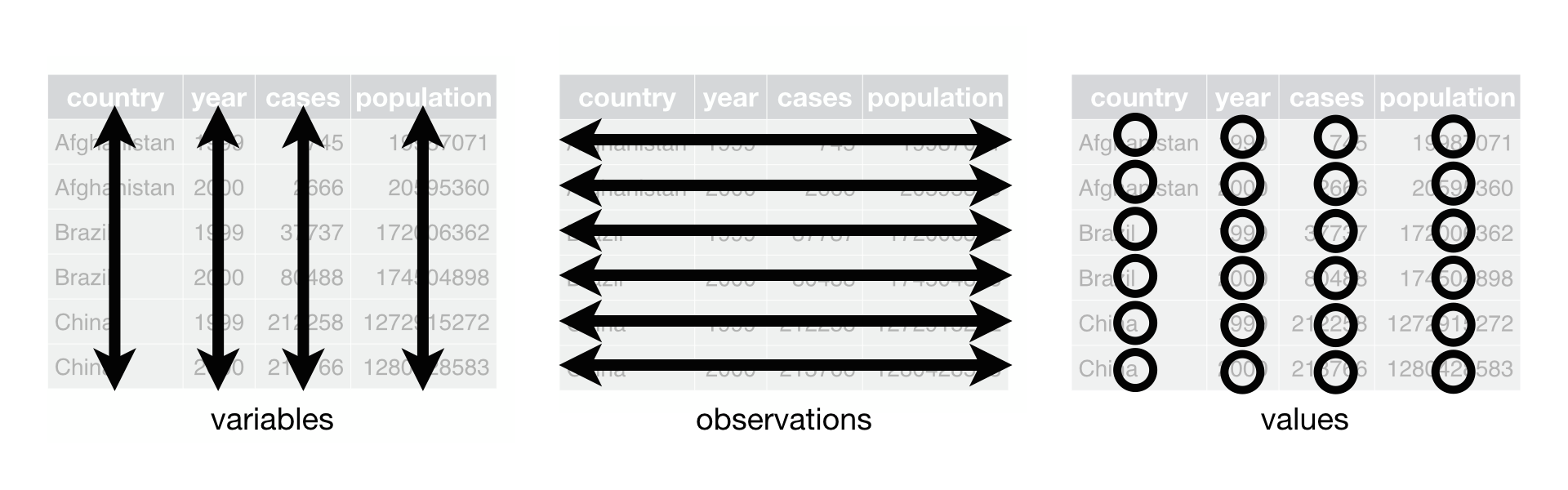
Each variable must have its own column
Each observation must have its own row
Each value must have its own cell

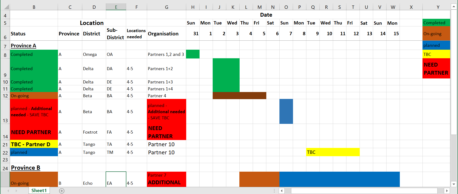
Excel data are often not tidy

We might be used to seeing data in “human readability” form
R cannot read this!

From The Epidemiologist R Handbook, Section 4.1

Let’s look at an example¹ of data represented in different ways

We will look at a dataset measuring tuberculosis (TB) cases for different countries. We have information on the country, year, population, and number of TB cases:

Each column is one piece of information:

# A tibble: 6 × 4
  country      year  cases population
  <chr>       <dbl>  <dbl>      <dbl>
1 Afghanistan  1999    745   19987071
2 Afghanistan  2000   2666   20595360
3 Brazil       1999  37737  172006362
4 Brazil       2000  80488  174504898
5 China        1999 212258 1272915272
6 China        2000 213766 1280428583

Population and cases are “types” of counts:

# A tibble: 12 × 4
   country      year type            count
   <chr>       <dbl> <chr>           <dbl>
 1 Afghanistan  1999 cases             745
 2 Afghanistan  1999 population   19987071
 3 Afghanistan  2000 cases            2666
 4 Afghanistan  2000 population   20595360
 5 Brazil       1999 cases           37737
 6 Brazil       1999 population  172006362
 7 Brazil       2000 cases           80488
 8 Brazil       2000 population  174504898
 9 China        1999 cases          212258
10 China        1999 population 1272915272
11 China        2000 cases          213766
12 China        2000 population 1280428583

We look at the rate of TB cases:

# A tibble: 6 × 3
  country      year rate             
  <chr>       <dbl> <chr>            
1 Afghanistan  1999 745/19987071     
2 Afghanistan  2000 2666/20595360    
3 Brazil       1999 37737/172006362  
4 Brazil       2000 80488/174504898  
5 China        1999 212258/1272915272
6 China        2000 213766/1280428583

Tidy data works best with R functions

Tidy data allow us to transform, summarize, and plot our data very easily!

Example: If we want to calculate the rate of TB for each country and year, we will be able to simply instruct R to calculate \[ \text{rate} = \dfrac{\text{cases}}{\text{population}}\]

Each column is one piece of information:

# A tibble: 6 × 4
  country      year  cases population
  <chr>       <dbl>  <dbl>      <dbl>
1 Afghanistan  1999    745   19987071
2 Afghanistan  2000   2666   20595360
3 Brazil       1999  37737  172006362
4 Brazil       2000  80488  174504898
5 China        1999 212258 1272915272
6 China        2000 213766 1280428583

Our HRS data are in tidy form

Each column is a piece of information for an individual in the dataset

tibble(hrs_data) |> print(n = 8)

# A tibble: 2,728 × 32
  hhid   pn    id    birthyr birthmo birthdate proxy coupled sex   age_mo age_yr
  <fct>  <fct> <chr>   <dbl>   <dbl>     <dbl> <fct> <fct>   <fct>  <dbl>  <dbl>
1 552754 010   5527…    1967       9      2814 Resp… Not a … Fema…    665     55
2 555339 020   5553…    1966       7      2387 Resp… Couple… Fema…    676     56
3 559734 010   5597…    1967       3      2602 Resp… Couple… Male     663     55
4 558143 020   5581…    1973      10      5036 Resp… Couple… Male     600     50
5 554789 020   5547…    1950       7     -3153 Resp… Couple… Male     860     71
6 551018 010   5510…    1970       1      3667 Resp… Not a … Fema…    632     52
7 550516 010   5505…    1960       1        14 Resp… Not a … Male     749     62
8 559093 010   5590…    1971       4      4122 Resp… Couple… Male     621     51
# ℹ 2,720 more rows
# ℹ 21 more variables: ed <dbl>, degree <fct>, race_original <fct>,
#   smoke_ever <fct>, smoke_now <fct>, drink <fct>, height <dbl>, srh <fct>,
#   act_vig <fct>, bp <fct>, diab <fct>, cancer <fct>, lung <fct>, hrt <fct>,
#   strk <fct>, psych <fct>, sleep <fct>, arth <fct>, cond_count <dbl>,
#   cesd <dbl>, income <dbl>

Wrap-up

Tidy data are especially useful in R!
We will see more of its advantages in later lessons