Missing data: summarization and visualization

Nicky Wakim, Jessica Minnier, and Meike Niederhausen

Before we start

• Install and load the naniar package (a play on Narnia) if you haven’t already!

Artwork by @allison_horst

• We’ll be working with only a few variables in the HRS dataset in this lesson!
  • Mostly to help us view the tables and plots within the slides

hrs_00 <- hrs_data |>
  select(ed, race_original, srh, sex, act_vig, height)

 

Why summarize and visualize missingness before doing anything else?

• Before you transform, model, or plot a variable, you need to know how much of it is actually there

 

Missing data can be a problem for many reasons

• It can reduce your sample size (and therefor your ability to make conclusions)
• It can bias your results if there’s a pattern to missingness
• It can make your plots look weird or misleading

A quick missingness check can reveal

• Which variables have the most missing data
• Whether missingness is scattered or clustered
• Whether missingness looks related to another variable (which matters for how you handle it later)

Missing values in a dataset

• n_miss() from naniar counts the total number of missing values across an entire dataset

n_miss(hrs_00)

[1] 1061

• This is the total count of NA cells across every column combined
• n_complete() is the complement of n_miss()
  • It counts the total number of non-missing values across the dataset

 

• prop_miss() gives the proportion of all cells in the dataset that are missing

prop_miss(hrs_00)

[1] 0.0648216

• Useful as a single, high-level number to report on the overall proportion missingness of your dataset

Missing values in a single variable

• We can use n_miss() to count the number of missing values in a single variable

n_miss(hrs_00$srh)

[1] 4

• This is the count of NA cells in self-reported health

 

• We can also use prop_miss() to get the proportion of missing values in a single variable

prop_miss(hrs_00$srh)

[1] 0.001466276

• This is the proportion of NA cells in self-reported health

Missingness by each variable, for every variable

• miss_var_summary() gives one row per variable, with the count and percent missing
• Piping the result into gt() makes it a nicer table to read

hrs_00 |>
  miss_var_summary() |>
  gt() |>
  tab_options(table.font.size = px(40))

variable	n_miss	pct_miss
ed	507	18.6
race_original	486	17.8
height	55	2.02
act_vig	9	0.330
srh	4	0.147
sex	0	0

• The output is sorted from most to least missing, which makes it easy to spot the variables with the most missing data

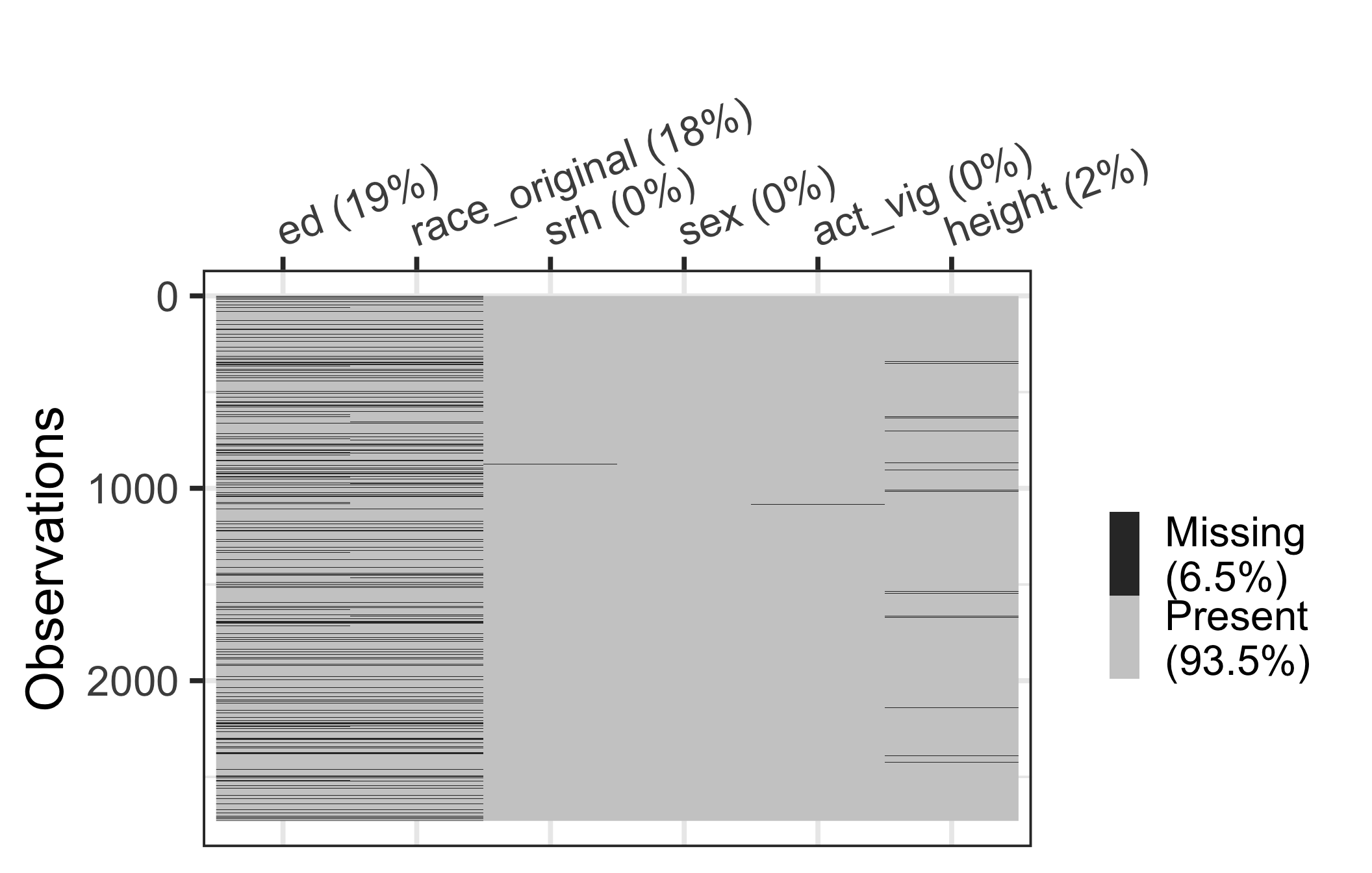
vis_miss(): visualizing missing data across the dataset

• This plot helps identify whether:
  • There are variables with a lot of missing values (in columns of plot)
  • Observations with a lot of missing values (in rows of plot)

 

hrs_00 |>
  vis_miss() +
  theme(axis.text.x = element_text(angle = 20, hjust = 0))

1

vis_miss() is a function with a lot of built-in defaults that will produce a plot showing the missingness of the dataset

2

I made some changes to the theme() to make the variable names easier to read

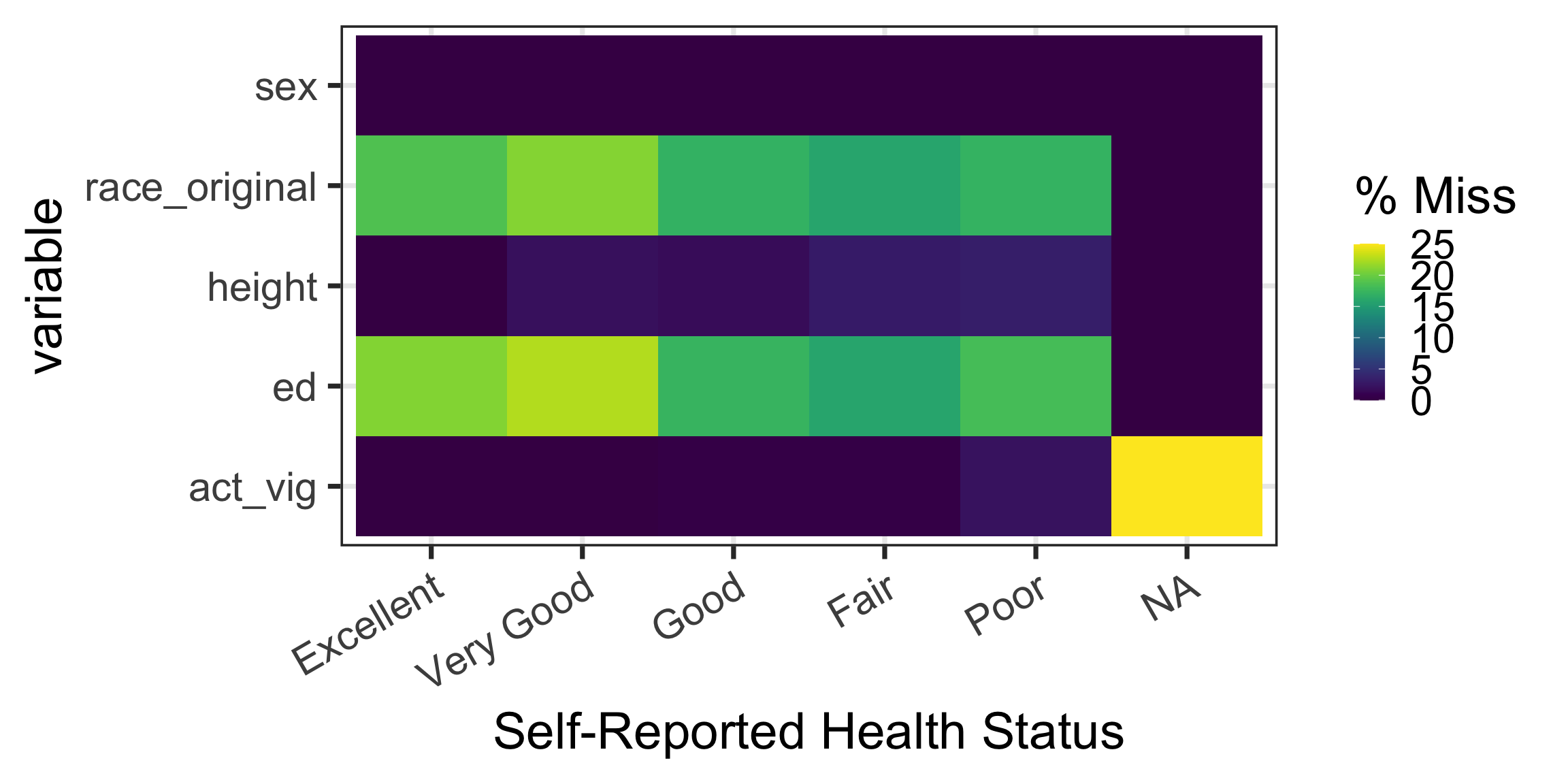
gg_miss_fct(): missingness heatmap by group

• This plot is useful for comparing missingness rates stratified by a variable
  • Potentially detect patterns in missingness
• Specify the variable to stratify by in the fct = option of gg_miss_fct()
  • Each column (x-axis) is a different level of the stratifying variable
  • Each row (y-axis) is a different variable in the dataset

Example: percent missingness stratified by srh (self-reported health)

hrs_00 |>
  gg_miss_fct(fct = srh) +
  theme_bw(base_size = 28) +
  theme(axis.text.x = element_text(angle = 30, hjust = 1))

1

gg_miss_fct() is a function that produces a heatmap of missingness stratified by a factor variable. We are stratifying by self-reported health (srh) in this example

2

I’m changing the background and font size to make the plot easier to read

3

I’m rotating the x-axis labels to make them easier to read

gg_miss_upset(): missingness intersections (1/2)

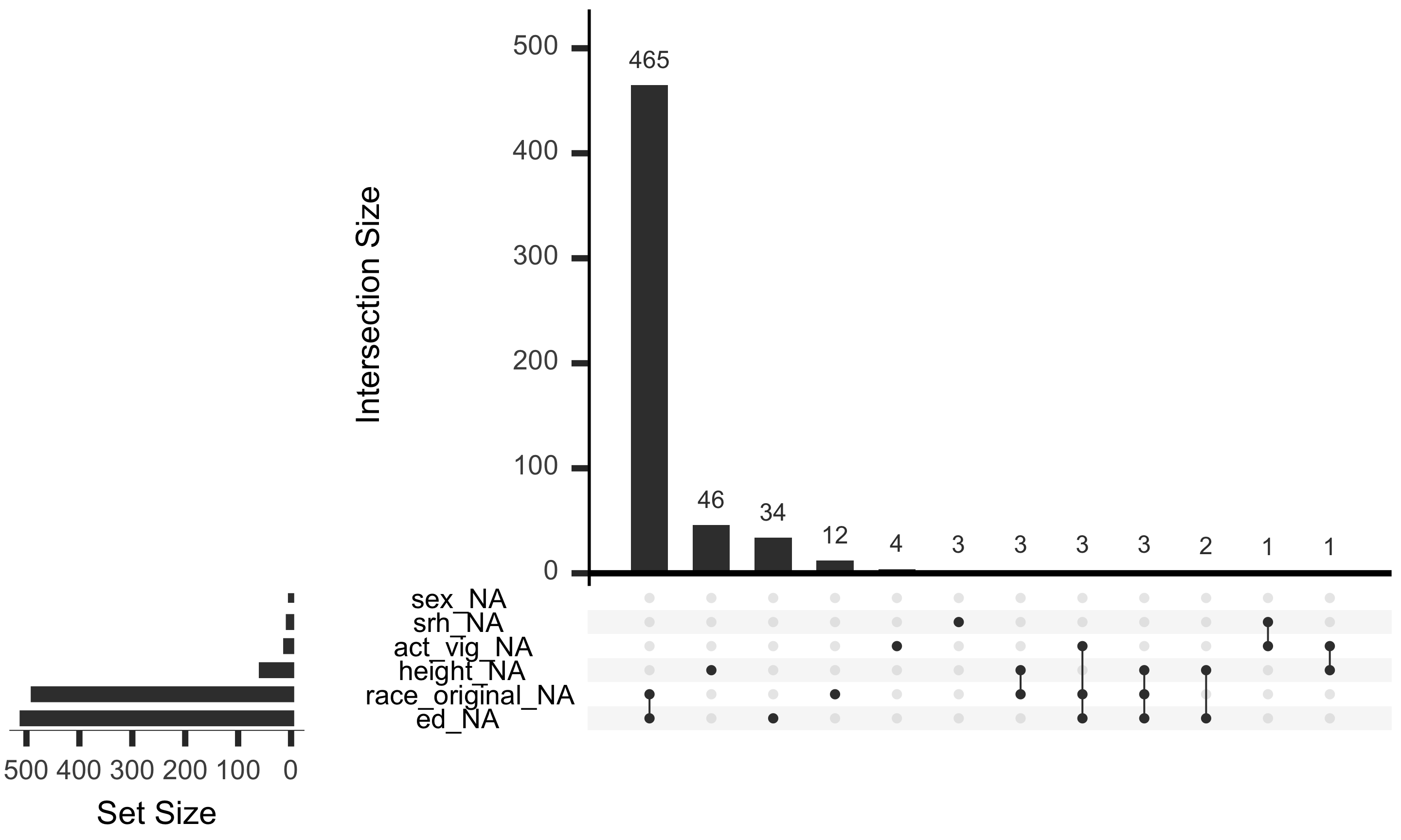
• gg_miss_upset() shows the most common combinations (sets) of missing variables

hrs_00 |>
  gg_miss_upset(
    nsets = 10,
    text.scale = 3
    )

1

gg_miss_upset() is a function that produces an UpSet plot of missingness intersections

2

nsets = 10 limits the plot to the 10 largest combinations of co-missing variables, which keeps the plot readable

3

text.scale = 3 increases the size of the text in the plot, which makes it easier to read

gg_miss_upset(): missingness intersections (2/2)

• gg_miss_upset() shows the most common combinations (sets) of missing variables

hrs_00 |>
  gg_miss_upset(
    nsets = 10,
    text.scale = 3
    )

1

gg_miss_upset() is a function that produces an UpSet plot of missingness intersections

2

nsets = 10 limits the plot to the 10 largest combinations of co-missing variables, which keeps the plot readable

3

text.scale = 3 increases the size of the text in the plot, which makes it easier to read

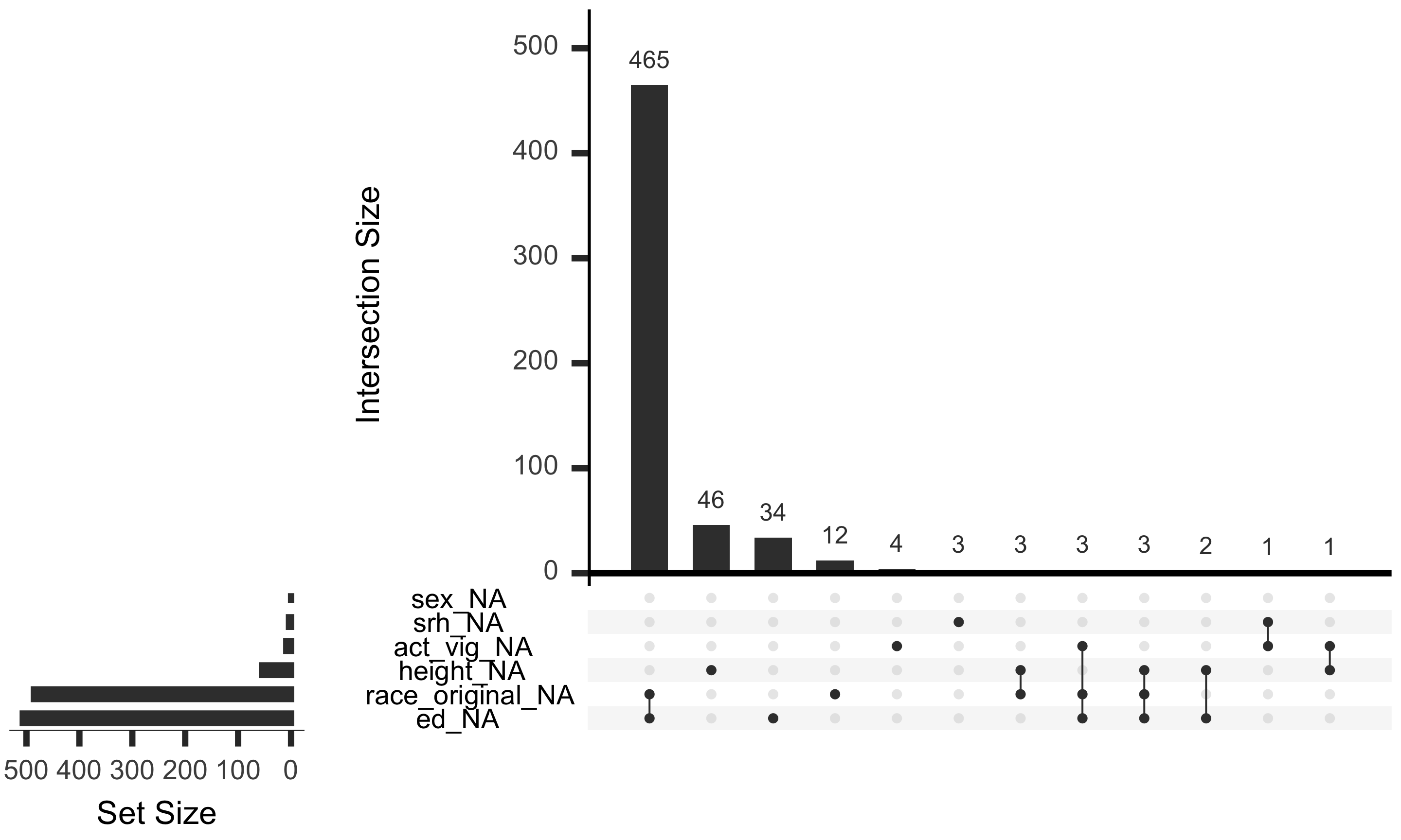
• Main bar plot: ordered by the number of observations with specific set of missing variables
• Bottom dots with lines: combination of variables missing
• Bottom, sideways barplot: number of observations missing for each variable, regardless of combination

gg_miss_upset(): What am I taking away from this plot?

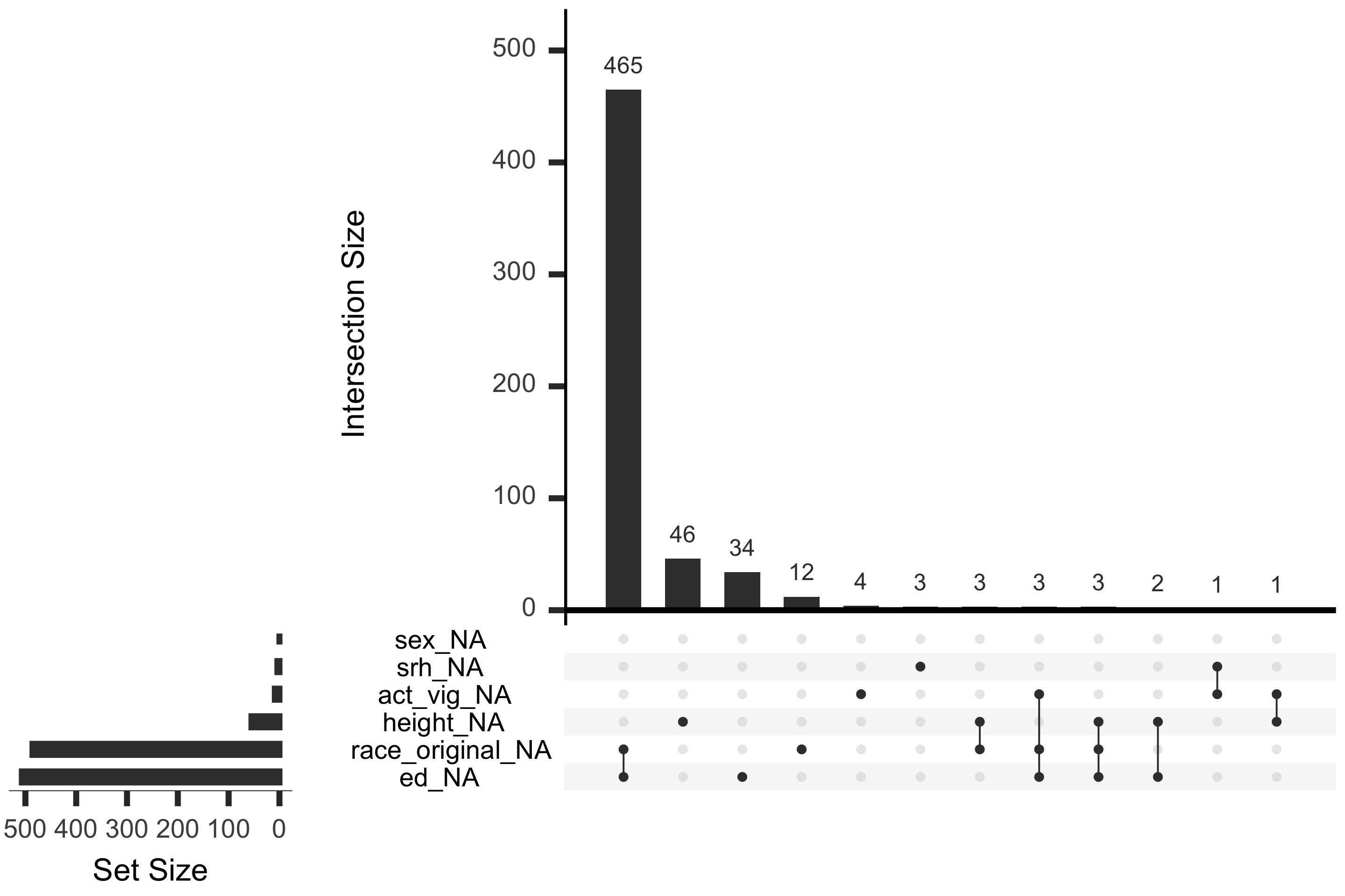
• The most common combination of missing variables is race_original and ed with 465 observations
  • There are not many observations that have one of these missing without the other
  • There’s 36 (34 + 2) observations that have ed missing but not race_original
  • There’s 15 (12 + 3) observations that have race_original missing but not ed
• Height seems to be mostly missing on its own
  • 46 out of the 55 observations with height missing have no other variables missing

Wrap-up

• We learned a few functions within naniar that help us summarize and visualize missingness in a dataset

 

• n_miss() and prop_miss() give quick, high-level counts of missingness across a whole dataset
• miss_var_summary() gives a tidy, sortable summary of missingness by variable
• vis_miss() gives a bird’s-eye view of missingness across every row and column
• gg_miss_fct() compares missingness rates across groups
• gg_miss_upset() reveals which variables tend to be missing together

Resources

• Exploring missing values in naniar: interactive tutorial
• {naniar} package website
• Missing values chapter in R for Data Science (2e)
• Dealing with missing data in the Epidemiologist R Handbook