Lesson 2: Introduction to Categorical Data Analysis

Nicky Wakim

2024-04-03

Learning Objectives

1. Recognize the motivation for and focus of our course (categorical responses)

2. Recall features of the Binomial distribution for categorical data analysis and utilize the normal approximation

3. Determine if a single proportion differs from a population value

4. Determine if two proportions differ from each other

5. Display data from two categorical variables, each with 2 or more categories, using R X C contingency tables

6. Determine if a nominal response and nominal explanatory variable are associated with one another using the Chi-squared test

7. Determine if a nominal response and nominal explanatory variable are associated with one another using the Fisher Exact test

8. Determine if a binary, nominal response and an ordinal explanatory variable are associated with one another using the Cochran-Armitage test

9. Determine if an ordinal response and ordinal explanatory variable are associated with one another using the Mantel-Haenszel test

Learning Objectives

1. Recognize the motivation for and focus of our course (categorical responses)

2. Recall features of the Binomial distribution for categorical data analysis and utilize the normal approximation

3. Determine if a single proportion differs from a population value

4. Determine if two proportions differ from each other

5. Display data from two categorical variables, each with 2 or more categories, using R X C contingency tables

6. Determine if a nominal response and nominal explanatory variable are associated with one another using the Chi-squared test

7. Determine if a nominal response and nominal explanatory variable are associated with one another using the Fisher Exact test

8. Determine if a binary, nominal response and an ordinal explanatory variable are associated with one another using the Cochran-Armitage test

9. Determine if an ordinal response and ordinal explanatory variable are associated with one another using the Mantel-Haenszel test

What is Categorical Data Analysis?

• In BSTA 512/612 (linear regression), we focused on continuous responses/outcomes

  • We included categorical variables only as covariates (aka predictors, independent variables, explanatory variables)

  • Examples from 512/612: life expectancy (in years), IAT score (ranging from -2 to 2)

   

• Categorical data analysis focuses on the statistical methods for categorical responses/outcomes

  • Explanatory (or ‘independent’) variable can be of any type (continuous or categorical)

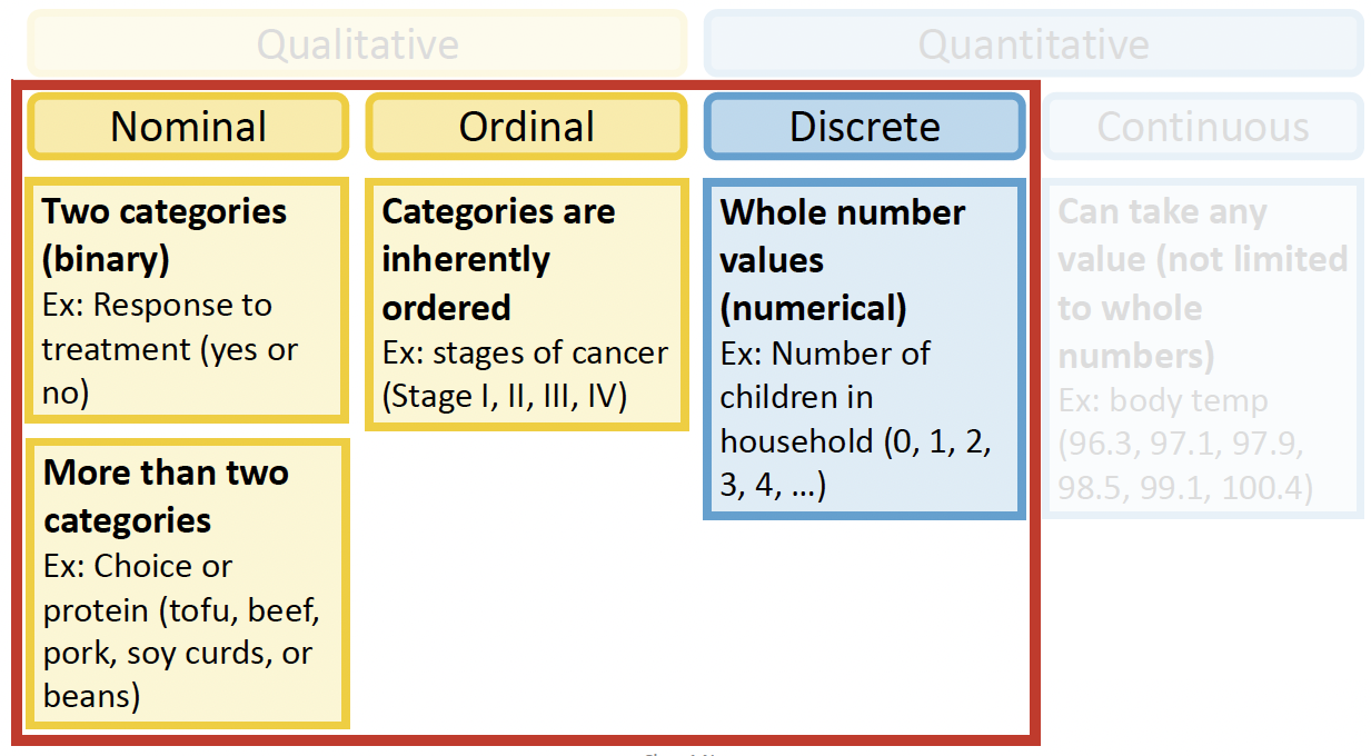
Types of Variables

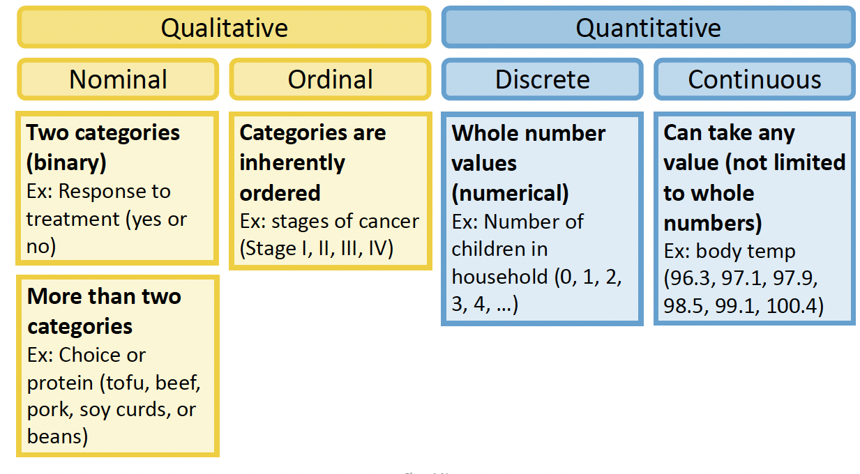
Types of Variables: Outcomes we will cover in this course

What does this course cover?

• Strategies for assessing association between categorical response variable and a one explanatory variable

  • Hypothesis testing
  • Measure of association
  • Simple logistic regression

   

• Statistical modeling strategies for assessing association between the categorical response variable and a set of explanatory variables

  • Logistic regression

    • For binary, ordinal, and multinomial outcomes

  • Poisson regression

    • For counts outcomes

Poll everywhere question 1

Learning Objectives

1. Recognize the motivation for and focus of our course (categorical responses)

2. Recall features of the Binomial distribution for categorical data analysis and utilize the normal approximation

3. Determine if a single proportion differs from a population value

4. Determine if two proportions differ from each other

5. Display data from two categorical variables, each with 2 or more categories, using R X C contingency tables

6. Determine if a nominal response and nominal explanatory variable are associated with one another using the Chi-squared test

7. Determine if a nominal response and nominal explanatory variable are associated with one another using the Fisher Exact test

8. Determine if a binary, nominal response and an ordinal explanatory variable are associated with one another using the Cochran-Armitage test

9. Determine if an ordinal response and ordinal explanatory variable are associated with one another using the Mantel-Haenszel test

Binomial Distribution

• Consider a sample of \(n\) independent trials, each of which can have only two possible outcomes (“success” and “failure”)

• For each trial: \[\begin{align} P( \text{success}) & = p \\ P( \text{failure}) & = 1- p = q \end{align}\]

• Binomial distribution: distribution of the number of successes in n independent trials

• The probability mass function for the binomial distribution is: \[P(X=k) = {n \choose k} p^k q^{n-k}, \text{ for } k = 0, 1, ..., n\]

  • \(E(X) = np\)
  • \(Var(X) = npq = np(1-p)\)

Binomial Distribution

• Consider a sample of \(n\) independent trials, each of which can have only two possible outcomes (“success” and “failure”)

• For each trial: \[\begin{align} P( \text{success}) & = p \\ P( \text{failure}) & = 1- p = q \end{align}\]

• Binomial distribution: distribution of the number of successes in n independent trials

• The probability mass function for the binomial distribution is: \[P(X=k) = {n \choose k} p^k q^{n-k}, \text{ for } k = 0, 1, ..., n\]

  • \(E(X) = np\)
  • \(Var(X) = npq = np(1-p)\)

Binomial Distribution: R commands

R commands with their input and output:

R code	What does it return?
rbinom()	returns sample of random variables with specified binomial distribution
dbinom()	returns probability of getting certain number of successes
pbinom()	returns cumulative probability of getting certain number or less successes
qbinom()	returns number of successes corresponding to desired quantile

Binomial Distribution Example

Example

If the probability that one white blood cell is a lymphocyte is 0.2, compute the probability of 2 lymphocytes out of 10 white blood cells

\[P(X=2) = {10 \choose 2} 0.2^2 (1-0.2)^{10-2} = 0.3020\]

dbinom(2, 10, 0.2) %>% round(4)

[1] 0.302

Normal Approximation of the Binomial Distribution

• Also known as: Sampling distribution of \(\widehat{p}\)

• IF \(X\sim \text{Binomial}(n,p)\) and \(np>10\) and \(nq = n(1-p) > 10\)

  • Ensures sample size (\(n\)) is moderately large and the \(p\) is not too close to 0 or 1
  • Other resources use other criteria (like \(npq>5\) or \(np>5\))
  • When looking at a sample, we use \(\widehat{p}\) instead of \(p\) to check this!!

 

• THEN approximately \(𝑋\sim \text{Normal}\big(\mu_X = np, \sigma_X = \sqrt{np(1-p)} \big)\)

  • Or we often write this as the sampling distribution of \(\widehat{p}\): \[\widehat{p} \sim \text{Normal}\bigg(\mu_{\widehat{p}} = p, \sigma_{\widehat{p}} = \sqrt{\dfrac{p(1-p)}{n}}\bigg)\]

• Pretty good video behind the intuition of this (Watch 00:00 - 05:40)

Learning Objectives

1. Recognize the motivation for and focus of our course (categorical responses)

2. Recall features of the Binomial distribution for categorical data analysis and utilize the normal approximation

3. Determine if a single proportion differs from a population value

4. Determine if two proportions differ from each other

5. Display data from two categorical variables, each with 2 or more categories, using R X C contingency tables

6. Determine if a nominal response and nominal explanatory variable are associated with one another using the Chi-squared test

7. Determine if a nominal response and nominal explanatory variable are associated with one another using the Fisher Exact test

8. Determine if a binary, nominal response and an ordinal explanatory variable are associated with one another using the Cochran-Armitage test

9. Determine if an ordinal response and ordinal explanatory variable are associated with one another using the Mantel-Haenszel test

Estimate and Confidence Interval of Single Proportion

• Estimate of proportion:

\[ \widehat{p} = \dfrac{\# \text{successes}}{\# \text{successes} + \# \text{failures}} \]

• Use the sampling distribution of \(\widehat{p}\) to construct the confidence interval:

  • \((1-\alpha)\%\) confidence interval for estimate proportion:

\[\begin{align} \widehat{p} &\pm z^*_{(1-\alpha/2)} \cdot SE_{\hat{p}} \\ \widehat{p} &\pm z^*_{(1-\alpha/2)} \cdot \sqrt{\frac{\hat{p}(1-\hat{p})}{n}} \end{align}\]

• Using \(SE_{\hat{p}} = \sqrt{\frac{\hat{p}(1-\hat{p})}{n}}\) - instead of \(\sigma_{p} = \sqrt{\frac{p(1-p)}{n}}\) - because we don’t know exactly what \(p\) is

Smoking status example

A cross-sectional study of 8681 patients was conducted to evaluate the nature of smoking status among people. Of the 8681 people, 4840 were nonsmokers and 3841 were smokers.

Needed steps:

1. Estimate proportion \(\widehat{p}\)
2. Check that \(n\widehat{p}>10\) and \(n(1-\widehat{p})>10\) in order to make normal approximation
3. Construct 95% confidence interval
4. Write interpretation

Smoking status example

A cross-sectional study of 8681 patients was conducted to evaluate the nature of smoking status among people. Of the 8681 people, 4840 were nonsmokers and 3841 were smokers.

1. Estimate proportion \(\widehat{p}\) \[ \widehat{p} = \dfrac{3841}{3841 + 4840} = \dfrac{3841}{8681} = 0.44246\]
2. Check that \(n\widehat{p}>10\) and \(n(1-\widehat{p})>10\) in order to make normal approximation \[ n\widehat{p} = 8681\cdot0.4425 = 3841 > 10\] \[ n(1-\widehat{p}) = 8681\cdot(1-0.4425) = 4840 > 10\]

3. Construct 95% confidence interval

\[ \widehat{p} \pm z^*_{0.975} \cdot \sqrt{\frac{\hat{p}(1-\hat{p})}{n}}\]

prop.test(x = 3841, n = 8681, correct = T)

    1-sample proportions test with continuity correction

data:  3841 out of 8681, null probability 0.5
X-squared = 114.73, df = 1, p-value < 2.2e-16
alternative hypothesis: true p is not equal to 0.5
95 percent confidence interval:
 0.4319827 0.4529896
sample estimates:
        p 
0.4424605 

4. Write interpretation of estimate

The estimated proportion of smokers is 0.442 (95% CI: 0.432, 0.453).

Additional interpretation of CI: We are 95% confident that the (population) proportion of smokers is between 0.432 and 0.453.

Poll everywhere question 2

Learning Objectives

1. Recognize the motivation for and focus of our course (categorical responses)

2. Recall features of the Binomial distribution for categorical data analysis and utilize the normal approximation

3. Determine if a single proportion differs from a population value

4. Determine if two proportions differ from each other

5. Display data from two categorical variables, each with 2 or more categories, using R X C contingency tables

6. Determine if a nominal response and nominal explanatory variable are associated with one another using the Chi-squared test

7. Determine if a nominal response and nominal explanatory variable are associated with one another using the Fisher Exact test

8. Determine if a binary, nominal response and an ordinal explanatory variable are associated with one another using the Cochran-Armitage test

9. Determine if an ordinal response and ordinal explanatory variable are associated with one another using the Mantel-Haenszel test

Estimate and Confidence Interval for Difference in Proportions

• Use the sampling distribution of \(\widehat{p}_1\) and \(\widehat{p}_2\) to construct the confidence interval:

  • \((1-\alpha)\%\) confidence interval for estimate difference in proportions:

\[\begin{align} \widehat{p}_1 - \widehat{p}_2 &\pm z^*_{(1-\alpha/2)} \cdot SE_{\hat{p}_1 - \hat{p}_2} \\ \widehat{p}_1 - \widehat{p}_2 &\pm z^*_{(1-\alpha/2)} \cdot \sqrt{ \frac{\hat{p}_1\cdot(1-\hat{p}_1)}{n_1} + \frac{\hat{p}_2\cdot(1-\hat{p}_2)}{n_2}} \end{align}\]

• Using \(SE_{\hat{p}_1 - \hat{p}_2} = \sqrt{\frac{\hat{p}_1\cdot(1-\hat{p}_1)}{n_1} + \frac{\hat{p}_2\cdot(1-\hat{p}_2)}{n_2}}\) because we don’t know exactly what \(p_1\) and \(p_2\) are

Poll Everywhere Question 3

Example: Strong Heart Study (1/2)

The Strong Heart Study is an ongoing study of American Indians residing in 13 tribal communities in three geographic areas (AZ, OK, and SD/ND) to study prevalence and incidence of cardiovascular disease and to identify risk factors. We will be examining the 4-year cumulative incidence of diabetes with one risk factor, glucose tolerance.

 

• Impaired glucose: normal or impaired glucose tolerance at baseline visit (between 1988 and 1991)

   

• Diabetes: Indicator of diabetes at follow-up visit (roughly four years after baseline) according to two-hour oral glucose tolerance test

Example: Strong Heart Study (2/2)

There is a total of 1664 American Indians in the dataset, with the following distribution of folks with diabetes and glucose tolerance:

 

#shs_data = read.csv(file = here("./data/SHS_data.csv"))

SHS = tibble(Diabetes = c(rep("Not diabetic", 
                   1338), 
                   rep("Diabetic", 326)),
              Glucose = c(rep("Normal", 
                  1004),#Not diabetic
          rep("Impaired", 334),
          rep("Normal", 
              128), #Diabetic
          rep("Impaired", 198)))

Displaying the contingency table in R

SHS %>% tabyl(Glucose, Diabetes) %>% 
  adorn_totals(where = c("row", "col")) %>% 
  gt() %>% 
  tab_stubhead(label = "Glucose Impairment") %>%
  tab_spanner(label = "Diabetes", 
              columns = c("Not diabetic", "Diabetic")) %>%
  tab_options(table.font.size = 45)

Glucose	Diabetes		Total
	Not diabetic	Diabetic
Impaired	334	198	532
Normal	1004	128	1132
Total	1338	326	1664

Strong Heart Study

What is the difference in proportions for American Indians that have diabetes comparing individuals with normal vs. impaired glucose?

Needed steps:

1. Estimate the difference in proportions
2. Check that each cell has at least 10 individuals
3. Construct 95% confidence interval
4. Write interpretation of estimate

Strong Heart Study

What is the difference in proportions for American Indians that have diabetes comparing individuals with normal vs. impaired glucose?

Glucose	Diabetes		Total
	Not diabetic	Diabetic
Impaired	334	198	532
Normal	1004	128	1132
Total	1338	326	1664

1. Estimate the difference in proportions \[ \widehat{p}_1 -\widehat{p}_2 = \dfrac{198}{532} - \dfrac{128}{1132} = 0.2591\]

2. Check that each cell has at least 10 individuals

3. Construct 95% confidence interval

prop.test(x = table(SHS$Glucose, SHS$Diabetes), 
          correct = T)

    2-sample test for equality of proportions with continuity correction

data:  table(SHS$Glucose, SHS$Diabetes)
X-squared = 152.6, df = 1, p-value < 2.2e-16
alternative hypothesis: two.sided
95 percent confidence interval:
 0.2126963 0.3055162
sample estimates:
   prop 1    prop 2 
0.3721805 0.1130742 

4. Write interpretation of estimate

The estimated difference in proportion of diabetic American Indians comparing is 0.259 (95% CI: 0.213, 0.306).

Additional interpretation of CI: We are 95% confident that the difference in (population) proportions of American Indians who have normal glucose tolerance and impaired glucose tolerance that developed diabetes is between 0.213 and 0.306.

McNemar’s Test

• McNemar’s test should be used if data is from a matched pairs study

 

• What is a matched-pairs study?

  • Participants are paired based on key characteristics
  • Each participant within a pair will be assigned to different treatment groups

• Categorical test that is parallel to the “paired t-test”

 

• R packages and functions

  • Normal approximation: mcnemar.test() in built-in stats package
  • Exact test: mcnemar.exact() in exact2x2 package

 

• If you would like more information of McNemar’s test, please see Rosner TB: 10.4 and 10.5: Paired Samples

Summary so far

• Introduced categorical data as the response in analysis
• Reviewed an important distribution (Binomial distribution) for categorical data analysis
• Estimated a single proportion from a sample with its confidence interval
• Estimated a difference in proportions from a sample with its confidence interval

   

• Can we expand this to ask a more general question about association between a response and explanatory variable?

  • What if there is more than 2 categories for either variable?

Learning Objectives

1. Recognize the motivation for and focus of our course (categorical responses)

2. Recall features of the Binomial distribution for categorical data analysis and utilize the normal approximation

3. Determine if a single proportion differs from a population value

4. Determine if two proportions differ from each other

5. Display data from two categorical variables, each with 2 or more categories, using R X C contingency tables

6. Determine if a nominal response and nominal explanatory variable are associated with one another using the Chi-squared test

7. Determine if a nominal response and nominal explanatory variable are associated with one another using the Fisher Exact test

8. Determine if a binary, nominal response and an ordinal explanatory variable are associated with one another using the Cochran-Armitage test

9. Determine if an ordinal response and ordinal explanatory variable are associated with one another using the Mantel-Haenszel test

Contingency Tables (R x C)

• R X C contingency tables

  • Contains information for two discrete variables: one has R categories and the other has C categories.

  • Refers to the number of rows (R) and number of columns (C) in the table

 

• For two proportions: focused on 2 X 2 contingency tables

  • R = 2, C = 2

 

• Expand our contingency tables to variables with 2 or more categories

  • Categories can be ordinal or nominal

Contingency Table: Example

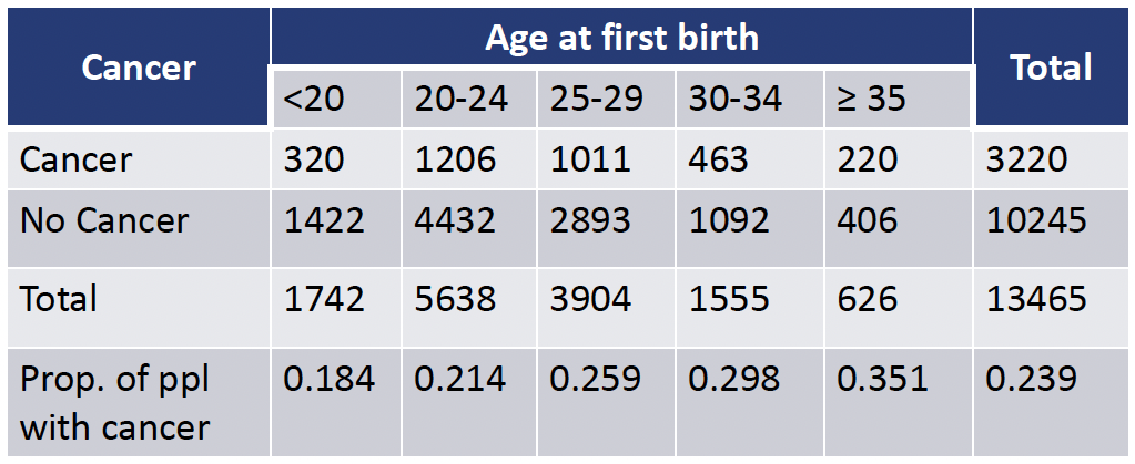
Let’s say we are interested in learning the association between the development of breast cancer and age at first birth. Our first step is typically to present the observed data:

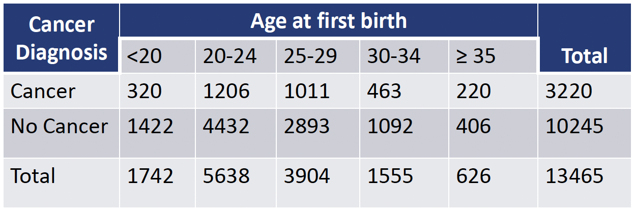
• This is a 2 x 5 contingency table

Test Association/Trend of R X C Contingency Table

 

If both variables are nominal, a test of general association will be sufficient

• Test of general association is the same regardless of R and C

• Test used for 2x2 contingency table same as 5x3 contingency table

• We will cover:

  • Chi-squared test
  • Fisher Exact test

If one or both variables are ordinal, a test of trend may be of interest

• Treats ordinal variables as quantitative rather than qualitative (nominal scale)

• Test of trend has greater power than the test of general association

• We will cover:

  • Cochran-Armitage test
  • Mantel-Haenszel test

Poll Everywhere Question 4

Test of General Association

• General research question: Are two variables (both categorical, nominal) associated with each other?

 

• Translated to a hypothesis test:

  • \(H_0\) : There is no association between the two variables / The variables are independent
  • \(H_1\) : There is an association between the two variables / The variables are not independent

   

• We have two options for testing general association:

  1. Chi-squared test
  2. Fisher’s Exact test

Test of General Association: SHS Example

• Main question: Do American Indians with impaired glucose tolerance have a different incidence of diabetes?

  • Is glucose tolerance associated with diabetes incidence among American Indians?

• We have two variables, and both variables have two nominal categories

  • Diabetes outcome: Not diabetic and Diabetic
  • Glucose tolerance: Normal or Impaired

 

• Answer research question with a test of general association

• Hypothesis:

  • \(H_0\) : There is no association between glucose tolerance and diabetes / Glucose tolerance and diabetes are independent
  • \(H_1\) : There is an association between glucose tolerance and diabetes / Glucose tolerance and diabetes are not independent

Learning Objectives

1. Recognize the motivation for and focus of our course (categorical responses)

2. Recall features of the Binomial distribution for categorical data analysis and utilize the normal approximation

3. Determine if a single proportion differs from a population value

4. Determine if two proportions differ from each other

5. Display data from two categorical variables, each with 2 or more categories, using R X C contingency tables

6. Determine if a nominal response and nominal explanatory variable are associated with one another using the Chi-squared test

7. Determine if a nominal response and nominal explanatory variable are associated with one another using the Fisher Exact test

8. Determine if a binary, nominal response and an ordinal explanatory variable are associated with one another using the Cochran-Armitage test

9. Determine if an ordinal response and ordinal explanatory variable are associated with one another using the Mantel-Haenszel test

Chi-squared test

• Test to see how likely is it that we observe our data given the null hypothesis (no association)

 

• We use the null to calculate the expected cell counts and compare them to the observed cell counts

 

• Requirements to conduct Chi-squared test (expected cell counts)

  • For 2 x 2 contingency table:

    • No expected cell counts should be less than 10

  • For contingency table with 3x2, 3x3, 4x4, etc.:

    • No more than 20% of expected cell counts are less than 5
    • No expected cell counts are less than 1

Chi-squared test: Process

1. Check that the expected cell counts threshold is met

2. Set the level of significance \(\alpha\)

3. Specify the null ( \(H_0\) ) and alternative ( \(H_A\) ) hypotheses

   • In symbols
   • In words
   • Alternative: one- or two-sided?

4. Calculate the test statistic and p-value for Chi-squared test in R

   • We will not discuss the test statistic’s equation

5. Write a conclusion to the hypothesis test

   • Do we reject or fail to reject \(H_0\)?
   • Write a conclusion in the context of the problem

Chi-squared test: Expected Cell Counts

• Is the sample size big enough for the chi-square test to be adequate? What are the expected cell counts?

 

• If you want an explanation of how to calculate by hand, please see Vu and Harringtion TB (section 8.3.1, page 405)

 

• Too time consuming for this class, but R does it quickly using the expected() function in the epitools package

Chi-squared test: Expected Cell Counts

• In the Strong Heart Study…

SHS_table = table(SHS$Glucose, SHS$Diabetes)
SHS_table

          
           Diabetic Not diabetic
  Impaired      198          334
  Normal        128         1004

library(epitools)
expected(SHS_table)

          
           Diabetic Not diabetic
  Impaired  104.226      427.774
  Normal    221.774      910.226

 

All expected counts > 5

Chi-squared test: SHS Example

1. Check expected cell counts threshold

expected(SHS_table)

          
           Diabetic Not diabetic
  Impaired  104.226      427.774
  Normal    221.774      910.226

All expected cells are greater than 5.

2. \(\alpha = 0.05\)

3. Hypothesis test:

   • \(H_0\) : There is no association between glucose tolerance and diabetes
   • \(H_1\) : There is an association between glucose tolerance and diabetes

4. Calculate the test statistic and p-value for Chi-squared test in R

chisq.test(x = SHS_table, correct = T)

    Pearson's Chi-squared test with Yates' continuity correction

data:  SHS_table
X-squared = 152.6, df = 1, p-value < 2.2e-16

5. Conclusion to the hypothesis test

We reject the null hypothesis that glucose tolerance and diabetes are not associated (\(p<2.2\cdot10^{-16}\)). There is sufficient evidence that glucose tolerance and diabetes incidence are associated among American Indians.

Learning Objectives

1. Recognize the motivation for and focus of our course (categorical responses)

2. Recall features of the Binomial distribution for categorical data analysis and utilize the normal approximation

3. Determine if a single proportion differs from a population value

4. Determine if two proportions differ from each other

5. Display data from two categorical variables, each with 2 or more categories, using R X C contingency tables

6. Determine if a nominal response and nominal explanatory variable are associated with one another using the Chi-squared test

7. Determine if a nominal response and nominal explanatory variable are associated with one another using the Fisher Exact test

8. Determine if a binary, nominal response and an ordinal explanatory variable are associated with one another using the Cochran-Armitage test

9. Determine if an ordinal response and ordinal explanatory variable are associated with one another using the Mantel-Haenszel test

Fisher’s Exact Test

• Only necessary when expected counts in one or more cells is less than 5
• Given row and column totals fixed, computes exact probability that we observe our data or more extreme data
• Consider a general 2 x 2 table:

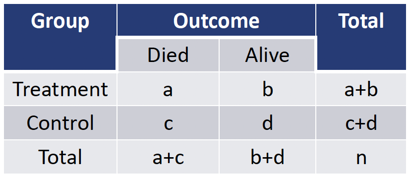
• The exact probability of observing a table with cells (a, b, c, d) can be computed based on the hypergeometric distribution

\[P(a, b, c, d) = \dfrac{(a+b)!\cdot(c+d)!\cdot(a+c)!\cdot(b+d)!}{n!\cdot a!\cdot b!\cdot c!\cdot d!}\]

• Numerator is fixed and denominator changes

Fisher’s Exact test: Process

1. Check the expected cell counts

2. Set the level of significance \(\alpha\)

3. Specify the null ( \(H_0\) ) and alternative ( \(H_A\) ) hypotheses

   • In symbols
   • In words
   • Alternative: one- or two-sided?

4. Calculate the test statistic and p-value for Fisher Exact test in R

   • We will not discuss the test statistic’s equation

5. Write a conclusion to the hypothesis test

   • Do we reject or fail to reject \(H_0\)?
   • Write a conclusion in the context of the problem

Fisher’s Exact test: SHS Example (not appropriate use of Fisher’s Exact)

1. Check expected cell counts threshold

expected(SHS_table)

          
           Diabetic Not diabetic
  Impaired  104.226      427.774
  Normal    221.774      910.226

We’re going to pretend they are less than 5.

2. \(\alpha = 0.05\)

3. Hypothesis test:

   • \(H_0\) : There is no association between glucose tolerance and diabetes
   • \(H_1\) : There is an association between glucose tolerance and diabetes

4. Calculate the test statistic and p-value for Chi-squared test in R

fisher.test(x = SHS_table)

    Fisher's Exact Test for Count Data

data:  SHS_table
p-value < 2.2e-16
alternative hypothesis: true odds ratio is not equal to 1
95 percent confidence interval:
 3.576595 6.048639
sample estimates:
odds ratio 
  4.644825 

5. Conclusion to the hypothesis test

We reject the null hypothesis that glucose tolerance and diabetes are not associated (\(p<2.2\cdot10^{-16}\)). There is sufficient evidence that glucose tolerance and diabetes incidence are associated among American Indians.

Learning Objectives

1. Recognize the motivation for and focus of our course (categorical responses)

2. Recall features of the Binomial distribution for categorical data analysis and utilize the normal approximation

3. Determine if a single proportion differs from a population value

4. Determine if two proportions differ from each other

5. Display data from two categorical variables, each with 2 or more categories, using R X C contingency tables

6. Determine if a nominal response and nominal explanatory variable are associated with one another using the Chi-squared test

7. Determine if a nominal response and nominal explanatory variable are associated with one another using the Fisher Exact test

8. Determine if a binary, nominal response and an ordinal explanatory variable are associated with one another using the Cochran-Armitage test

9. Determine if an ordinal response and ordinal explanatory variable are associated with one another using the Mantel-Haenszel test

Test of Trend

• If one or both variables are ordinal, a test of trend may be of interest

  • Treats ordinal variables as quantitative rather than qualitative (nominal scale)
  • Test of trend has greater power than the test of general association
  • You can use a test of general association for non-ordinal variables

 

• Two tests of trend that we we learn:

  • Cochran-Armitage test

    • Tests association between a binary response and an ordinal explanatory variable

  • Mantel-Haenszel test

    • Test association between an ordinal response and an ordinal explanatory variable

Cochran-Armitage test

• Cochran-Armitage test for trend will determine if there is association between a binary response variable and an ordinal variable with 3 or more categories

 

• It will test the trend of the proportions over the ordinal variable

  • Answers the question: Does the proportion of people with a “successful” outcome increase as the ordinal explanatory variable increases?

 

• Cochran-Armitage test for trend is only suitable for 2 x C contingency tables

Cochran-Armitage test: Hypothesis Test

Null Hypothesis (\(H_0\))

The proportions of successes are the same across all C ordinal values of the explanatory variable. \[p_1 = p_2 = ... = p_C\]

Alternative Hypothesis (\(H_1\))

The proportions of successes tend to increase as ordinal value of the explanatory variable increases

\[p_1 \leq p_2 \leq ... \leq p_C\]

OR

The proportions of successes tend to decrease as ordinal value of the explanatory variable increases

\[p_1 \geq p_2 \geq ... \geq p_C\]

Cochran-Armitage test: Process

1. Set the level of significance \(\alpha\)

2. Specify the null ( \(H_0\) ) and alternative ( \(H_A\) ) hypotheses

   • In symbols
   • In words
   • Alternative: one- or two-sided?

3. Calculate the test statistic and p-value for Cochran-Armitage test in R

   • We will not discuss the test statistic’s equation
   • Just know it follows a Normal distribution

4. Write a conclusion to the hypothesis test

   • Do we reject or fail to reject \(H_0\)?
   • Write a conclusion in the context of the problem

Cochran-Armitage test: Example (1/3)

We are interested in learning the association between the development of breast cancer and age at first birth among people who have given birth

       

   

Cochran-Armitage test: Example (2/3)

• Before we go into the hypothesis test procedure, we need to construct the contingency table in R

Cancer = c(320, 1206, 1011, 463, 220)
No_Cancer = c(1422, 4432, 2893, 1092, 406)
bscancer = matrix (c(Cancer, No_Cancer), nrow = 2, byrow = T)
rownames(bscancer) = c("Cancer","No Cancer")
colnames(bscancer) = c("<20","20-24","25-29","30-34",">=35")
bscancer

           <20 20-24 25-29 30-34 >=35
Cancer     320  1206  1011   463  220
No Cancer 1422  4432  2893  1092  406

• It does not need to be pretty to use in function

Cochran-Armitage test: Example (3/3)

1. \(\alpha = 0.05\)

2. Hypothesis test:

   • \(H_0\): The proportions of breast cancer are the same for all age levels of first birth. \[p_1 = p_2 = ... = p_5\]
   • \(H_1\): The proportions of breast cancer tends to increase as level of age of first birth increases

\[p_1 \leq p_2 \leq ... \leq p_5\]

3. Calculate the test statistic and p-value for Cochran-Armitage test in R

library(DescTools)
CochranArmitageTest(bscancer)

    Cochran-Armitage test for trend

data:  bscancer
Z = 11.358, dim = 5, p-value < 2.2e-16
alternative hypothesis: two.sided

4. Conclusion to the hypothesis test

We reject the null hypothesis that proportions of breast cancer are the same for all age levels of first birth (\(p<2.2\cdot10^{-16}\)). There is sufficient evidence that the proportion of of breast cancer increase as the the age at first birth increases.

Learning Objectives

1. Recognize the motivation for and focus of our course (categorical responses)

2. Recall features of the Binomial distribution for categorical data analysis and utilize the normal approximation

3. Determine if a single proportion differs from a population value

4. Determine if two proportions differ from each other

5. Display data from two categorical variables, each with 2 or more categories, using R X C contingency tables

6. Determine if a nominal response and nominal explanatory variable are associated with one another using the Chi-squared test

7. Determine if a nominal response and nominal explanatory variable are associated with one another using the Fisher Exact test

8. Determine if a binary, nominal response and an ordinal explanatory variable are associated with one another using the Cochran-Armitage test

9. Determine if an ordinal response and ordinal explanatory variable are associated with one another using the Mantel-Haenszel test

Mantel-Haenszel test

• When both variables are ordinal, we can conduct Mantel-Haenszel test of trend for linear association

• Mantel-Haenszel test for linear trend is suitable for any R x C contingency tables with two ordinal variables

• Hypothesis test:

Null Hypothesis (\(H_0\))

There is no correlation between the two variables \[ \rho = 0\]

Alternative Hypothesis (\(H_1\))

There is correlation between the two variables

\[ \rho \neq 0\]

Mantel-Haenszel test: Process

1. Set the level of significance \(\alpha\)

2. Specify the null ( \(H_0\) ) and alternative ( \(H_A\) ) hypotheses

   • In symbols
   • In words
   • Alternative: one- or two-sided?

3. Calculate the test statistic and p-value for Mantel-Haenszel test in R

   • We will not discuss the test statistic’s equation

4. Write a conclusion to the hypothesis test

   • Do we reject or fail to reject \(H_0\)?
   • Write a conclusion in the context of the problem

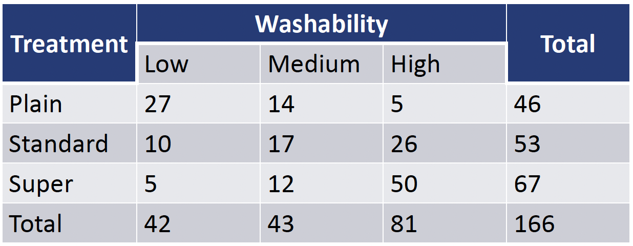
Mantel-Haenszel test: Example (1/3)

A water treatment company is studying water additives and investigating how they affect clothes washing (through measurements of abrasions, wearing, and color loss).

The treatments studies where no treatment (plain water), the standard treatment, and a double dose of the standard treatment, called super. Washability was measured as low, medium and high.

Are levels of washability associated with treatment?

 

 

Mantel-Haenszel test: Example (2/3)

• Before we go into the hypothesis test procedure, we need to construct the contingency table in R

water = matrix (c(27, 14, 5, 10, 17, 26, 5, 12, 50), nrow = 3, byrow = T)
rownames(water) = c("plain","standard","super")
colnames(water) = c("low","medium","high")
water

         low medium high
plain     27     14    5
standard  10     17   26
super      5     12   50

• It does not need to be pretty to use in function

Mantel-Haenszel test: Example (3/3)

1. \(\alpha = 0.05\)

2. Hypothesis test:

   • \(H_0\): Water treatment and washability are not correlated. \[ \rho = 0\]
   • \(H_1\): Water treatment and washability are correlated.

\[ \rho \neq 0\]

3. Calculate the test statistic and p-value for Mantel-Haenszel test in R

library(DescTools)
MHChisqTest(water)

    Mantel-Haenszel Chi-Square

data:  water
X-squared = 50.602, df = 1, p-value = 1.132e-12

4. Conclusion to the hypothesis test

We reject the null hypothesis that there is no correlation between washability and water treatment (\(p = 1.13 \cdot 10^{-12} < 0.05\)). There is sufficient evidence that level of water treatment is associated with washability.

Learning Objectives

1. Recognize the motivation for and focus of our course (categorical responses)

2. Recall features of the Binomial distribution for categorical data analysis and utilize the normal approximation

3. Determine if a single proportion differs from a population value

4. Determine if two proportions differ from each other

5. Display data from two categorical variables, each with 2 or more categories, using R X C contingency tables

6. Determine if a nominal response and nominal explanatory variable are associated with one another using the Chi-squared test

7. Determine if a nominal response and nominal explanatory variable are associated with one another using the Fisher Exact test

8. Determine if a binary, nominal response and an ordinal explanatory variable are associated with one another using the Cochran-Armitage test

9. Determine if an ordinal response and ordinal explanatory variable are associated with one another using the Mantel-Haenszel test

More resources

• For a refresher or review of one proportion and differences in proportions

  • And their power calculations

  • From Meike’s BSTA 511 course (see Day 12!)

• For a refresher or review of Chi-squared test or Fisher’s Exact test

  • From Meike’s BSTA 511 course (see Day 13!)