Lesson 3: Measurement of Association for Contingency Tables

Nicky Wakim

2024-04-08

Poll Everywhere Question 1

Make sure to remember your answer!! We’ll use this on Wednesday!

Learning Objectives

Understand the difference between testing for association and measuring association
Estimate the risk difference (and its confidence interval) from a contingency table and interpret the estimate.
Estimate the risk ratio (and its confidence interval) from a contingency table and interpret the estimate.
Estimate the odds ratio (and its confidence interval) from a contingency table and interpret the estimate.

Learning Objectives

Understand the difference between testing for association and measuring association

Estimate the risk difference (and its confidence interval) from a contingency table and interpret the estimate.
Estimate the risk ratio (and its confidence interval) from a contingency table and interpret the estimate.
Estimate the odds ratio (and its confidence interval) from a contingency table and interpret the estimate.

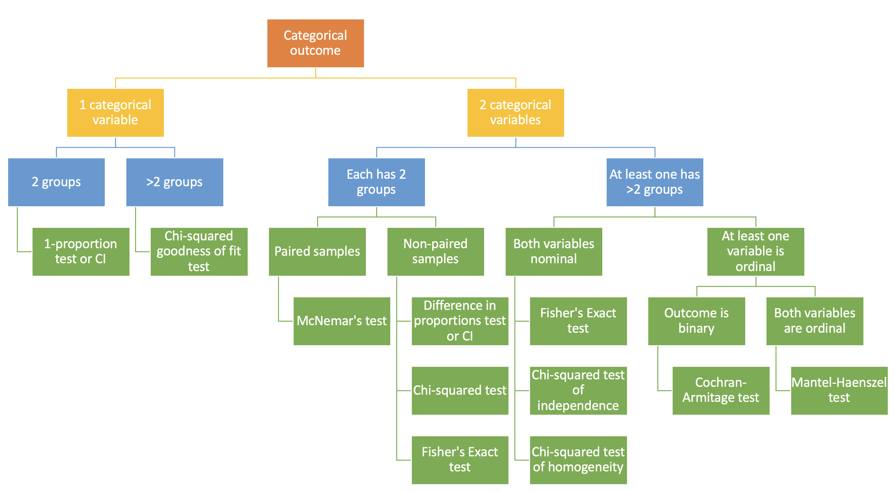
Review of Test of Association (1/2)

Last week: learned some tests of association for contingency tables

For studies with two independent samples
- General association
  - Chi-squared test
  - Fisher’s Exact test
- Test of trends
  - Cochran-Armitage test
  - Mantel-Haenszel test

Review of Test of Association (2/2)

Test of association does not measure association

Test of association does not provide an effective measure of association. The p-value alone is not enough
- $\text{p-value} < 0.05$ suggests there is a statistically significant association between the group and outcome
- $\text{p-value} = 0.00001$ vs. $\text{p-value} = 0.01$ does not mean the magnistude of association is different

But it does not tell how different the risks are between the two groups

We want to find out one or more measurements for quantifying the risks across the groups.

Measures of Association

When we have a 2x2 contingency table and independent samples, we have an option of three measures of association:
1. Risk difference (RD)
1. Relative risk (RR)
1. Odds ratio (OR)

Each measures association by comparing the proportion of successes/failures from each categorical group of our explanatory variable.

Before we discuss each further…

Let’s define the cells within a 2x2 contingency table:

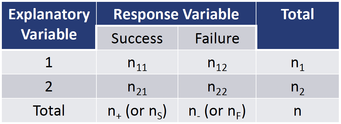
Then we can define risk: the proportion of “successes”
- With $\text{Risk}_1 = \dfrac{n_{11}}{n_1}$

Learning Objectives

Understand the difference between testing for association and measuring association

Estimate the risk difference (and its confidence interval) from a contingency table and interpret the estimate.

Estimate the risk ratio (and its confidence interval) from a contingency table and interpret the estimate.
Estimate the odds ratio (and its confidence interval) from a contingency table and interpret the estimate.

Risk Difference (RD)

Risk difference computes the absolute difference in risk for the two groups (from the explanatory variable)
Point estimate: \[\widehat{RD} = \widehat{p}_1 - \widehat{p}_1 = \dfrac{n_{11}}{n_1} - \dfrac{n_{21}}{n_2}\]
- With range of point estimate from $[-1, 1]$
Approximate standard error:

\[ SE_{\widehat{RD}} = \sqrt{\frac{\hat{p}_1\cdot(1-\hat{p}_1)}{n_1} + \frac{\hat{p}_2\cdot(1-\hat{p}_2)}{n_2}}\]

95% Wald confidence interval for $\widehat{RD}$:

\[\widehat{RD} \pm 1.96 \cdot SE_{\widehat{RD}}\]

Recall the Strong Heart Study

The Strong Heart Study is an ongoing study of American Indians residing in 13 tribal communities in three geographic areas (AZ, OK, and SD/ND). We will look at data from this study examining the incidence of diabetes at a follow-up visit and impaired glucose tolerance (ITG) at baseline (4 years apart).

Glucose tolerance	Diabetes		Total
Glucose tolerance	No	Yes	Total
Impaired	334	198	532
Normal	1004	128	1132
Total	1338	326	1664

SHS Example: Risk Difference

Risk difference

Compute the point estimate and 95% confidence interval for the diabetes risk difference between impaired and normal glucose tolerance.

Glucose tolerance	Diabetes		Total
Glucose tolerance	No	Yes	Total
Impaired	334	198	532
Normal	1004	128	1132
Total	1338	326	1664

Needed steps:

Compute the risk difference
Compute 95% confidence interval
Interpret the estimate

SHS Example: Risk Difference (1/4)

Risk difference

Compute the point estimate and 95% confidence interval for the diabetes risk difference between impaired and normal glucose tolerance.

Glucose tolerance	Diabetes		Total
Glucose tolerance	No	Yes	Total
Impaired	334	198	532
Normal	1004	128	1132
Total	1338	326	1664

Compute the risk difference \[\widehat{RD}={\hat{p}}_1 - {\hat{p}}_2=\frac{n_{11}}{n_1}-\frac{n_{21}}{n_2}=\ \frac{198}{532}\ - \frac{128}{1132}=0.3722−0.1131=0.2591\]

SHS Example: Risk Difference (2/4)

Risk difference

Compute the point estimate and 95% confidence interval for the diabetes risk difference between impaired and normal glucose tolerance.

Glucose tolerance	Diabetes		Total
Glucose tolerance	No	Yes	Total
Impaired	334	198	532
Normal	1004	128	1132
Total	1338	326	1664

Compute 95% confidence interval

\[\begin{aligned} &\widehat{RD}\pm z_{\left(1-\frac{\alpha}{2}\right)}^\ast \times SE_{\widehat{RD}} \\ = &\widehat{RD}\pm z_{\left(1-\frac{\alpha}{2}\right)}^\ast \times \sqrt{\frac{{\hat{p}}_1\ (1-{\hat{p}}_1)}{n_1}+\frac{{\hat{p}}_2(1-{\hat{p}}_2)}{n_2}\ }\\ = & 0.2591 \pm 1.96\times \sqrt{\frac{0.3722(1-0.3722)}{532}+\frac{0.1131(1-0.1131)}{1132}\ }\\ = & (0.2141,\ 0.3041 )\end{aligned}\]

SHS Example: Risk Difference (3/4)

Risk difference

Compute the point estimate and 95% confidence interval for the diabetes risk difference between impaired and normal glucose tolerance.

Glucose tolerance	Diabetes		Total
Glucose tolerance	No	Yes	Total
Impaired	334	198	532
Normal	1004	128	1132
Total	1338	326	1664

1/2. Compute risk difference and 95% confidence interval

fmsb::riskdifference(198, 128, 532, 1132)

                 Cases People at risk         Risk
Exposed    198.0000000    532.0000000    0.3721805
Unexposed  128.0000000   1132.0000000    0.1130742
Total      326.0000000   1664.0000000    0.1959135


    Risk difference and its significance probability (H0: The difference
    equals to zero)

data:  198 128 532 1132
p-value < 2.2e-16
95 percent confidence interval:
 0.2140779 0.3041346
sample estimates:
[1] 0.2591062

SHS Example: Risk Difference (4/4)

Risk difference

Compute the point estimate and 95% confidence interval for the diabetes risk difference between impaired and normal glucose tolerance.

Glucose tolerance	Diabetes		Total
Glucose tolerance	No	Yes	Total
Impaired	334	198	532
Normal	1004	128	1132
Total	1338	326	1664

Interpret the estimate

The diabetes diagnosis risk difference between impaired and normal glucose tolerance is 0.2591 (95% CI: 0.2141, 0.3041). Since the 95% confidence interval contains 0, we do not have sufficient evidence that the risk of diabetes diagnosis between impaired and normal glucose tolerance is different.

When is the risk difference misleading?

The same risk differences can have very different clinical meanings depending on the risk for each group

Example: for two treatments A and B, we know the risk difference (RD) is 0.009. Is it a meaningful difference?
- If the risk is 0.01 for Trt A and 0.001 for Trt B?
- If the risk is 0.41 for Trt A and 0.401 for Trt B?

Using the RD alone to summarize the difference in risks for comparing the two groups can be misleading
- The ratio of risk can provide an informative descriptive measure of the “relative risk”

Learning Objectives

Understand the difference between testing for association and measuring association
Estimate the risk difference (and its confidence interval) from a contingency table and interpret the estimate.

Estimate the risk ratio (and its confidence interval) from a contingency table and interpret the estimate.

Estimate the odds ratio (and its confidence interval) from a contingency table and interpret the estimate.

Relative Risk (RR)

Relative risk computes the ratio of each group’s proportions of “success”
- Also called risk ratio
Point estimate: \[\widehat{RR}=\dfrac{\hat{p}_1}{\hat{p}_2} = \dfrac{n_{11}/n_1}{n_{21}/n_2}\]
- Range: $[0, \infty]$

Poll Everywhere Question 2

Log-transformation of RR

Sampling distribution of the relative risk is highly skewed unless sample sizes are quite large
- Log transformation results in approximately normal distribution
- Thus, compute confidence interval using normally distributed, log-transformed RR
- Then we convert back to the RR
We take the log (natural log) of RR: $\ln(\widehat{RR})$ or $log(\widehat{RR})$
- Whenever I say “log” I mean natural log (very common in statistics)

Then we need to find approximate standard error for $\ln(\widehat{RR})$ \[SE_{\ln(\widehat{RR})}=\sqrt{\frac{1}{n_{11}}\ -\frac{1}{n_1}+\frac{1}{n_{21}}-\frac{1}{n_2}}\]
95% confidence interval for $\ln(\widehat{RR})$: \[\ln(\widehat{RR}) \pm 1.96 \times SE_{\ln(\widehat{RR})}\]

How do we get back to the RR scale?

We computed confidence interval using normally distributed, log-transformed RR ($\ln(\widehat{RR})$):

\[ \bigg(\ln(\widehat{RR}) - 1.96 \times SE_{\ln(\widehat{RR})}, \ \ln(\widehat{RR}) + 1.96 \times SE_{\ln(\widehat{RR})}\bigg)\]

Now we need to exponentiate the CI to get back to interpretable values
- Take exponential of lower and upper bounds
95% confidence interval for RR: two ways to display equation

\[ \bigg(e^{\ln(\widehat{RR}) - 1.96 \times SE_{\ln(\widehat{RR})}}, \ e^{\ln(\widehat{RR}) + 1.96 \times SE_{\ln(\widehat{RR})}}\bigg)\] \[ \bigg(\exp\big(\ln(\widehat{RR}) - 1.96 \times SE_{\ln(\widehat{RR})}\big), \ \exp\big(\ln(\widehat{RR}) + 1.96 \times SE_{\ln(\widehat{RR})}\big)\bigg)\]

Relative Risk (RR)

Can you compute the estimated RRs for the previous example?
- If the risk for Trt A is 0.01 and Trt B is 0.001? $\widehat{RR}= 10$
- If the risk for Trt A is 0.41 and Trt B is 0.401? $\widehat{RR}= 1.02$
When $\widehat{RR}= 1$ …
- Risk is the same for the two groups
- In other words, the group and the outcome are independent
When computing $\widehat{RR}$ it is important to identify which variable is the response variable and which is explanatory variable
- We may say “risk for Trt A” but this translates to the risk (or probability) of outcome success for those receiving Trt A

SHS Example: Relative Risk (1/6)

Relative risk

Compute the point estimate and 95% confidence interval for the diabetes Relative risk between impaired and normal glucose tolerance.

Glucose tolerance	Diabetes		Total
Glucose tolerance	No	Yes	Total
Impaired	334	198	532
Normal	1004	128	1132
Total	1338	326	1664

Needed steps:

Compute the relative risk
Find confidence interval of log RR
Convert back to RR
Interpret the estimate

SHS Example: Relative Risk (2/6)

Relative risk

Compute the point estimate and 95% confidence interval for the diabetes Relative risk between impaired and normal glucose tolerance.

Glucose tolerance	Diabetes		Total
Glucose tolerance	No	Yes	Total
Impaired	334	198	532
Normal	1004	128	1132
Total	1338	326	1664

Compute the relative risk \[\widehat{RR}=\dfrac{{\hat{p}}_1}{{\hat{p}}_2}=\dfrac{n_{11}/{n_1}}{n_{21}/{n_2}}=\ \frac{ 198/532}{128/1132}=\dfrac{0.3722}{0.1131}=3.2915\]

SHS Example: Relative Risk (3/6)

Relative risk

Compute the point estimate and 95% confidence interval for the diabetes Relative risk between impaired and normal glucose tolerance.

Glucose tolerance	Diabetes		Total
Glucose tolerance	No	Yes	Total
Impaired	334	198	532
Normal	1004	128	1132
Total	1338	326	1664

Find confidence interval of log RR

\[\begin{aligned} & \ln(\widehat{RR}) \pm 1.96 \times SE_{\ln(\widehat{RR})} \\ = &\ln(\widehat{RR}) \pm z_{\left(1-\frac{\alpha}{2}\right)}^\ast \times \sqrt{\frac{1}{n_{11}}\ -\frac{1}{n_1}+\frac{1}{n_{21}}-\frac{1}{n_2}}\\ = & 1.1913 \pm 1.96\times \sqrt{\frac{1}{198}\ -\frac{1}{532}+\frac{1}{128}-\frac{1}{1132}}\\ = & (0.9944,\ 1.3883 )\end{aligned}\]

SHS Example: Relative Risk (4/6)

Relative risk

Compute the point estimate and 95% confidence interval for the diabetes Relative risk between impaired and normal glucose tolerance.

Glucose tolerance	Diabetes		Total
Glucose tolerance	No	Yes	Total
Impaired	334	198	532
Normal	1004	128	1132
Total	1338	326	1664

Convert back to RR

\[\begin{aligned} & (\exp(0.9944),\ \exp(1.3883 )) \\ = & (2.703,\ 4.0081 )\end{aligned}\]

SHS Example: Relative Risk (5/6)

Relative risk

Compute the point estimate and 95% confidence interval for the diabetes Relative risk between impaired and normal glucose tolerance.

Glucose tolerance	Diabetes		Total
Glucose tolerance	No	Yes	Total
Impaired	334	198	532
Normal	1004	128	1132
Total	1338	326	1664

1/2/3. Compute risk ratio and 95% confidence interval

library(epitools)
SHS_ct = table(SHS$glucimp, SHS$case)
riskratio(x = SHS_ct, rev = "rows")$measure

          risk ratio with 95% C.I.
           estimate    lower    upper
  Normal   1.000000       NA       NA
  Impaired 3.291471 2.702998 4.008061

Pause: other option in `pubh` package

SHS = SHS %>% mutate(glucimp = as.factor(glucimp) %>% relevel(ref = "Normal"))
contingency(case ~ glucimp, data = SHS)

          Outcome
Predictor     1    0
  Impaired  198  334
  Normal    128 1004

             Outcome +    Outcome -      Total                 Inc risk *
Exposed +          198          334        532     37.22 (33.10 to 41.48)
Exposed -          128         1004       1132      11.31 (9.52 to 13.30)
Total              326         1338       1664     19.59 (17.71 to 21.58)

Point estimates and 95% CIs:
-------------------------------------------------------------------
Inc risk ratio                                 3.29 (2.70, 4.01)
Inc odds ratio                                 4.65 (3.61, 6.00)
Attrib risk in the exposed *                   25.91 (21.41, 30.41)
Attrib fraction in the exposed (%)            69.62 (63.00, 75.05)
Attrib risk in the population *                8.28 (5.63, 10.94)
Attrib fraction in the population (%)         42.28 (34.71, 48.98)
-------------------------------------------------------------------
Uncorrected chi2 test that OR = 1: chi2(1) = 154.239 Pr>chi2 = <0.001
Fisher exact test that OR = 1: Pr>chi2 = <0.001
 Wald confidence limits
 CI: confidence interval
 * Outcomes per 100 population units 


    Pearson's Chi-squared test with Yates' continuity correction

data:  dat
X-squared = 152.6, df = 1, p-value < 2.2e-16

SHS Example: Relative Risk (6/6)

Relative risk

Compute the point estimate and 95% confidence interval for the diabetes Relative risk between impaired and normal glucose tolerance.

Glucose tolerance	Diabetes		Total
Glucose tolerance	No	Yes	Total
Impaired	334	198	532
Normal	1004	128	1132
Total	1338	326	1664

Interpret the estimate

The estimated risk of diabetes is 3.29 times greater for American Indians who had impaired glucose tolerance at baseline compared to those who had normal glucose tolerance (95% CI: 2.70, 4.01).

Additional interpretation of 95% CI (not needed): We are 95% confident that the (population) relative risk is between 2.70 and 4.01.

Since the 95% confidence interval does not include 1, there is sufficient evidence that the risk of diabetes differs significantly between impaired and normal glucose tolerance at baseline.

Learning Objectives

Understand the difference between testing for association and measuring association
Estimate the risk difference (and its confidence interval) from a contingency table and interpret the estimate.
Estimate the risk ratio (and its confidence interval) from a contingency table and interpret the estimate.

Estimate the odds ratio (and its confidence interval) from a contingency table and interpret the estimate.

Odds (building up to Odds Ratio)

For a probability of success $p$ (or sometimes referred to as $\pi$), the odds of success is: \[\text{odds}=\frac{p}{1-p}=\frac{\pi}{1-\pi}\]
- Example: if $\pi=0.75$, then odds of success $= \dfrac{0.75}{0.25}=3$
If odds > 1, it implies a success is more likely than a failure
- Example: for $odds = 3$, we expect to observe three times as many successes as failures
If odds is known, the probability of success can be computed \[\pi = \dfrac{\text{odds}}{\text{odds}+1}\]

Odds Ratio (OR)

Odds ratio is the ratio of two odds:\[\widehat{OR}=\frac{odds_1}{odds_2}=\frac{{\hat{p}}_1/(1-{\hat{p}}_1)}{{\hat{p}}_2/(1-{\hat{p}}_2)}\]
- Range: $[0, \infty]$
- Interpretation: The odds of success for “group 1” is “$\widehat{OR}$” times the odds of success for “group 2”

What do values of odds ratios mean?

Odds Ratio	Clinical Meaning
$\widehat{OR} < 1$	Odds of success is smaller in group 1 than in group 2
$\widehat{OR} = 1$	Explanatory and response variables are independent
$\widehat{OR} > 1$	Odds of success is greater in group 1 than in group 2

Poll Everywhere Question 3

Odds Ratio (OR)

Values of OR farther from 1.0 in a given direction represent stronger association
- An OR = 4 is farther from independence than an OR = 2
- An OR = 0.25 is farther from independence than an OR = 0.5
- For OR = 4 and OR = 0.25, they are equally away from independence (because ¼ = 0.25)

We take the inverse of the OR for success of group 1 compared to group 2 to get…
- OR for failure of group 1 compared to group 2
- OR for success of group 2 compared to group 1

Log-transformation of OR

Like RR, sampling distribution of the odds ratio is highly skewed
- Log transformation results in approximately normal distribution
- Thus, compute confidence interval using normally distributed, log-transformed OR

Approximate standard error for $\ln (\widehat{OR})$: \[SE_{\ln(\widehat{OR})}=\sqrt{\frac{1}{n_{11}}\ +\frac{1}{n_{12}}+\frac{1}{n_{21}}+\frac{1}{n_{22}}}\]
95% confidence interval for $\ln(\widehat{OR})$: \[\ln(\widehat{OR}) \pm 1.96 \times SE_{\ln(\widehat{OR})}\]

How do we get back to the OR scale?

We computed confidence interval using normally distributed, log-transformed RR ($\ln(\widehat{OR})$):

\[ \bigg(\ln(\widehat{OR}) - 1.96 \times SE_{\ln(\widehat{OR})}, \ \ln(\widehat{OR}) + 1.96 \times SE_{\ln(\widehat{OR})}\bigg)\]

Now we need to exponentiate the CI to get back to interpretable values
- Take exponential of lower and upper bounds
95% confidence interval for RR: two ways to display equation

\[ \bigg(e^{\ln(\widehat{OR}) - 1.96 \times SE_{\ln(\widehat{OR})}}, \ e^{\ln(\widehat{OR}) + 1.96 \times SE_{\ln(\widehat{OR})}}\bigg)\] \[ \bigg(\exp\big(\ln(\widehat{OR}) - 1.96 \times SE_{\ln(\widehat{OR})}\big), \ \exp\big(\ln(\widehat{OR}) + 1.96 \times SE_{\ln(\widehat{OR})}\big)\bigg)\]

SHS Example: Odds Ratio (1/6)

Odds ratio

Compute the point estimate and 95% confidence interval for the diabetes odds ratio between impaired and normal glucose tolerance.

Glucose tolerance	Diabetes		Total
Glucose tolerance	No	Yes	Total
Impaired	334	198	532
Normal	1004	128	1132
Total	1338	326	1664

Needed steps:

Compute the odds ratio
Find confidence interval of log OR
Convert back to OR
Interpret the estimate

SHS Example: Odds Ratio (2/6)

Odds ratio

Compute the point estimate and 95% confidence interval for the diabetes Odds ratio between impaired and normal glucose tolerance.

Glucose tolerance	Diabetes		Total
Glucose tolerance	No	Yes	Total
Impaired	334	198	532
Normal	1004	128	1132
Total	1338	326	1664

Compute the odds ratio

$\widehat{p}_1 = 198/532 = 0.3722$, $\widehat{p}_2 = 128/1132 = 0.1131$ \[\widehat{OR}=\frac{\widehat{p_1}/(1-\widehat{p_1})}{\widehat{p_2}/(1-\widehat{p_2})}= \dfrac{0.3722/(1-0.3722)}{0.1131/(1-0.1131)}= 4.6499\]

SHS Example: Odds Ratio (3/6)

Odds ratio

Compute the point estimate and 95% confidence interval for the diabetes Odds ratio between impaired and normal glucose tolerance.

Glucose tolerance	Diabetes		Total
Glucose tolerance	No	Yes	Total
Impaired	334	198	532
Normal	1004	128	1132
Total	1338	326	1664

Find confidence interval of log OR

\[\begin{aligned} & \ln(\widehat{OR}) \pm 1.96 \times SE_{\ln(\widehat{OR})} \\ = &\ln(\widehat{OR}) \pm z_{\left(1-\frac{\alpha}{2}\right)}^\ast \times \sqrt{\frac{1}{n_{11}}\ +\frac{1}{n_{12}}+\frac{1}{n_{21}}+\frac{1}{n_{22}}}\\ = & 1.5368 \pm 1.96\times \sqrt{\frac{1}{198}\ +\frac{1}{334}+\frac{1}{128}+\frac{1}{1004}}\\ = & (1.2824,\ 1.7913 )\end{aligned}\]

SHS Example: Odds Ratio (4/6)

Odds ratio

Compute the point estimate and 95% confidence interval for the diabetes Odds ratio between impaired and normal glucose tolerance.

Glucose tolerance	Diabetes		Total
Glucose tolerance	No	Yes	Total
Impaired	334	198	532
Normal	1004	128	1132
Total	1338	326	1664

Convert back to OR

\[\begin{aligned} & (\exp(1.2824),\ \exp(1.7913 )) \\ = & (3.6053,\ 5.9971 )\end{aligned}\]

SHS Example: Odds Ratio (5/6)

Odds ratio

Compute the point estimate and 95% confidence interval for the diabetes Odds ratio between impaired and normal glucose tolerance.

Glucose tolerance	Diabetes		Total
Glucose tolerance	No	Yes	Total
Impaired	334	198	532
Normal	1004	128	1132
Total	1338	326	1664

1/2/3. Compute OR and 95% confidence interval

library(epitools)
SHS_ct = table(SHS$glucimp, SHS$case)
# no `rev` needed below bc we set the reference level in slide 32
oddsratio(x = SHS_ct, method = "wald")$measure

          odds ratio with 95% C.I.
           estimate    lower    upper
  Normal   1.000000       NA       NA
  Impaired 4.649888 3.605289 5.997148

Pause: other option in `pubh` package

contingency(case ~ glucimp, data = SHS, digits = 3)

          Outcome
Predictor     1    0
  Impaired  198  334
  Normal    128 1004

             Outcome +    Outcome -      Total                 Inc risk *
Exposed +          198          334        532  37.218 (33.097 to 41.482)
Exposed -          128         1004       1132   11.307 (9.521 to 13.298)
Total              326         1338       1664  19.591 (17.709 to 21.581)

Point estimates and 95% CIs:
-------------------------------------------------------------------
Inc risk ratio                                 3.291 (2.703, 4.008)
Inc odds ratio                                 4.650 (3.605, 5.997)
Attrib risk in the exposed *                   25.911 (21.408, 30.413)
Attrib fraction in the exposed (%)            69.618 (63.004, 75.050)
Attrib risk in the population *                8.284 (5.631, 10.937)
Attrib fraction in the population (%)         42.284 (34.713, 48.976)
-------------------------------------------------------------------
Uncorrected chi2 test that OR = 1: chi2(1) = 154.239 Pr>chi2 = <0.001
Fisher exact test that OR = 1: Pr>chi2 = <0.001
 Wald confidence limits
 CI: confidence interval
 * Outcomes per 100 population units 


    Pearson's Chi-squared test with Yates' continuity correction

data:  dat
X-squared = 152.6, df = 1, p-value < 2.2e-16

SHS Example: Odds Ratio (6/6)

Odds ratio

Compute the point estimate and 95% confidence interval for the diabetes Odds ratio between impaired and normal glucose tolerance.

Glucose tolerance	Diabetes		Total
Glucose tolerance	No	Yes	Total
Impaired	334	198	532
Normal	1004	128	1132
Total	1338	326	1664

Interpret the estimate

The estimated odds of diabetes for American Indians with impaired glucose tolerance at baseline is 4.65 times the odds for American Indians with normal glucose tolerance at baseline.

Additional interpretation of 95% CI (not needed): We are 95% confident that the odds ratio is between 3.61 and 6.00.

Since the 95% confidence interval does not include 1, there is sufficient evidence that the odds of diabetes differs significantly between impaired and normal glucose tolerance at baseline.

Inversing an Odds Ratio

Some clinicians may prefer interpretations of OR > 1 instead of an OR < 1
The transformation can easily be done by inverse
- Remember we discussed that OR = 4 is an equivalent a strong association as OR = 0.25 (1/4)
OR comparing group 1 to group 2 = inverse of OR comparing group 2 to group 1

\[ OR_{1v2}=\frac{{\hat{p}}_1/(1-{\hat{p}}_1)}{{\hat{p}}_2/(1-{\hat{p}}_2)}=\frac{1}{\frac{{\hat{p}}_2/(1-{\hat{p}}_2)}{{\hat{p}}_1/(1-{\hat{p}}_1)}}=\frac{1}{OR_{2v1}}\]

Poll Everywhere Question 4

SHS Example: Inversing Odds Ratio

Inversing odds ratio

Compute the point estimate and 95% confidence interval for the diabetes odds ratio between normal and impaired glucose tolerance.

Glucose tolerance	Diabetes		Total
Glucose tolerance	No	Yes	Total
Impaired	334	198	532
Normal	1004	128	1132
Total	1338	326	1664

Needed steps:

Inverse point estimate and confidence interval

\[\widehat{OR}=\frac{1}{4.6499}=0.2151\] The 95% Confidence interval is then

\[ \left(\frac{1}{5.9971}, \frac{1}{3.6053}\right)\ =\ (0.1667, 0.2774)\]

SHS Example: Inversing Odds Ratio

Inversing odds ratio

Compute the point estimate and 95% confidence interval for the diabetes odds ratio between normal and impaired glucose tolerance.

Glucose tolerance	Diabetes		Total
Glucose tolerance	No	Yes	Total
Impaired	334	198	532
Normal	1004	128	1132
Total	1338	326	1664

Needed steps:

Inverse point estimate and confidence interval

library(epitools)
oddsratio(x = SHS_ct, method = "wald", rev = "rows")$measure

          odds ratio with 95% C.I.
           estimate     lower     upper
  Impaired 1.000000        NA        NA
  Normal   0.215059 0.1667459 0.2773702

SHS Example: Inversing Odds Ratio

Inversing odds ratio

Compute the point estimate and 95% confidence interval for the diabetes odds ratio between normal and impaired glucose tolerance.

Glucose tolerance	Diabetes		Total
Glucose tolerance	No	Yes	Total
Impaired	334	198	532
Normal	1004	128	1132
Total	1338	326	1664

Needed steps:

Interpret the estimate

The estimated odds of diabetes for American Indians with normal glucose tolerance at baseline is 0.22 times the odds for American Indians with impaired glucose tolerance at baseline.

Additional interpretation of 95% CI (not needed): We are 95% confident that the odds ratio is between 0.17 and 0.28.

Since the 95% confidence interval does not include 1, there is sufficient evidence that the odds of diabetes differs significantly between impaired and normal glucose tolerance at baseline.

Learning Objectives

Understand the difference between testing for association and measuring association
Estimate the risk difference (and its confidence interval) from a contingency table and interpret the estimate.
Estimate the risk ratio (and its confidence interval) from a contingency table and interpret the estimate.
Estimate the odds ratio (and its confidence interval) from a contingency table and interpret the estimate.

`pubh` vs. `epitools`

In pubh with contingency()
- Get all the info at once
- Really nice to double check how the code is interpreting your input
In epitools with riskratio() or oddsratio()
- Much easier to grab the numbers!
- In Quarto you can take R code and directly put it in your text
```
g = oddsratio(x = SHS_ct, method = "wald", rev = "rows")
g$measure[2,1]
```
```
[1] 0.215059
```
  - I can write {r eval="false" echo="true"} round(g$measure[2,1], 3) to print the number 0.215

Odds Ratio	Clinical Meaning
\(\widehat{OR} < 1\)	Odds of success is smaller in group 1 than in group 2
\(\widehat{OR} = 1\)	Explanatory and response variables are independent
\(\widehat{OR} > 1\)	Odds of success is greater in group 1 than in group 2

Lesson 3: Measurement of Association for Contingency Tables

Poll Everywhere Question 1

Learning Objectives

Learning Objectives

Review of Test of Association (1/2)

Review of Test of Association (2/2)

Test of association does not measure association

Measures of Association

Before we discuss each further…

Learning Objectives

Risk Difference (RD)

Recall the Strong Heart Study

SHS Example: Risk Difference

SHS Example: Risk Difference (1/4)

SHS Example: Risk Difference (2/4)

SHS Example: Risk Difference (3/4)

SHS Example: Risk Difference (4/4)

When is the risk difference misleading?

Learning Objectives

Relative Risk (RR)

Poll Everywhere Question 2

Log-transformation of RR

How do we get back to the RR scale?

Relative Risk (RR)

SHS Example: Relative Risk (1/6)

SHS Example: Relative Risk (2/6)

SHS Example: Relative Risk (3/6)

SHS Example: Relative Risk (4/6)

SHS Example: Relative Risk (5/6)

Pause: other option in pubh package

SHS Example: Relative Risk (6/6)

Learning Objectives

Odds (building up to Odds Ratio)

Odds Ratio (OR)

Poll Everywhere Question 3

Odds Ratio (OR)

Log-transformation of OR

How do we get back to the OR scale?

SHS Example: Odds Ratio (1/6)

SHS Example: Odds Ratio (2/6)

SHS Example: Odds Ratio (3/6)

SHS Example: Odds Ratio (4/6)

SHS Example: Odds Ratio (5/6)

Pause: other option in pubh package

SHS Example: Odds Ratio (6/6)

Inversing an Odds Ratio

Poll Everywhere Question 4

SHS Example: Inversing Odds Ratio

SHS Example: Inversing Odds Ratio

SHS Example: Inversing Odds Ratio

Learning Objectives

pubh vs. epitools

Pause: other option in `pubh` package

Pause: other option in `pubh` package

`pubh` vs. `epitools`