Lesson 6: Tests for GLMs using Likelihood function
2024-04-17
Revisit the likelihood function
Likelihood function: expresses the probability of the observed data as a function of the unknown parameters
- Function that enumerates the likelihood (similar to probability) that we observe the data across the range of potential values of our coefficients
We often compare likelihoods to see what estimates are more likely given our data
Plot to right is a simplistic view of likelihood
- I have flattened the likelihood that would be a function of \(\beta_0\) and \(\beta_1\) into a 2D plot (instead of 3D: \(\beta_0\) vs. \(\beta_1\) vs. \(L(\beta_0, \beta_1)\))
I use \(L\) to represent the log-likelihood and \(l\) to represent the likelihood

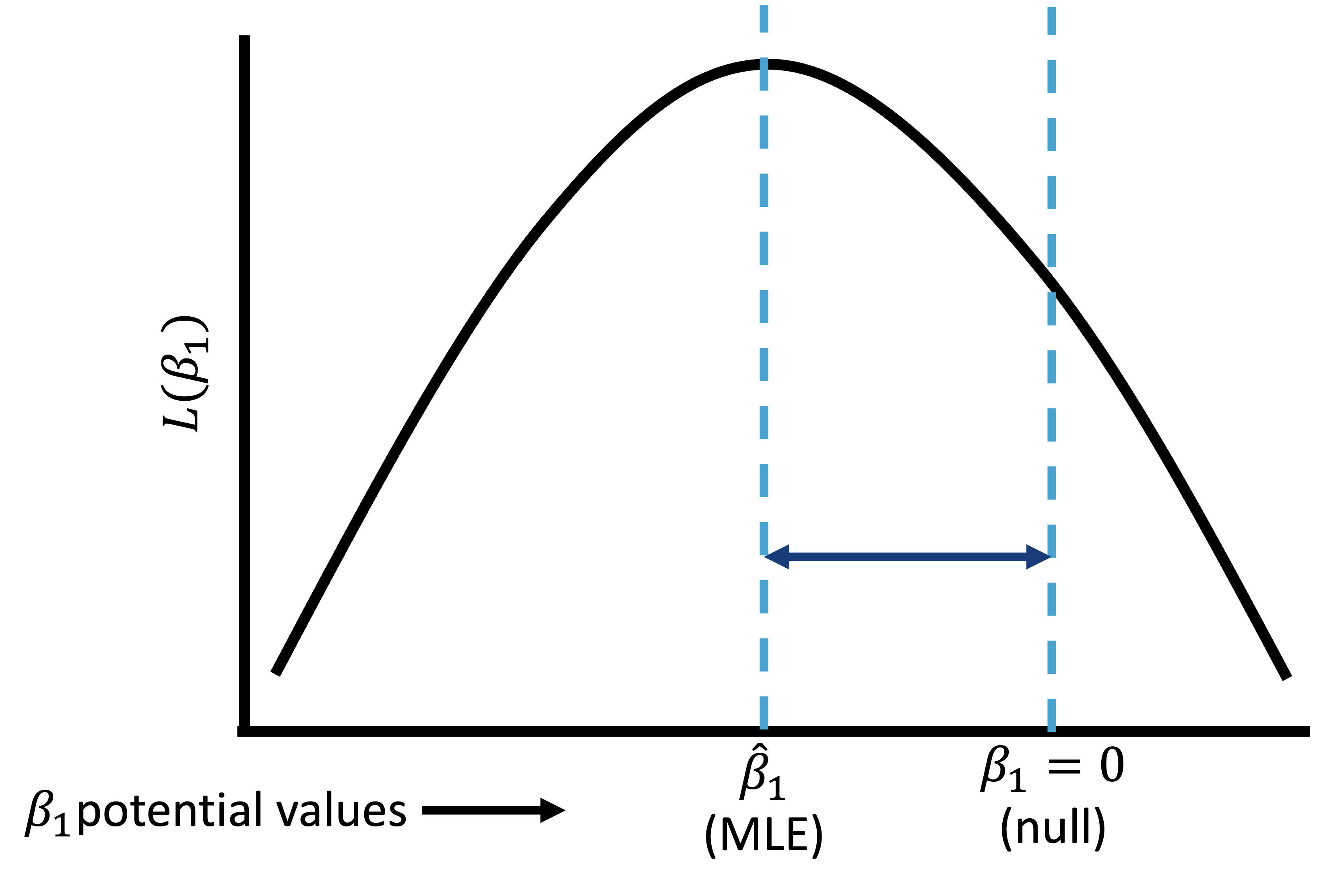
Wald test (2/3)
Wald test (3/3)
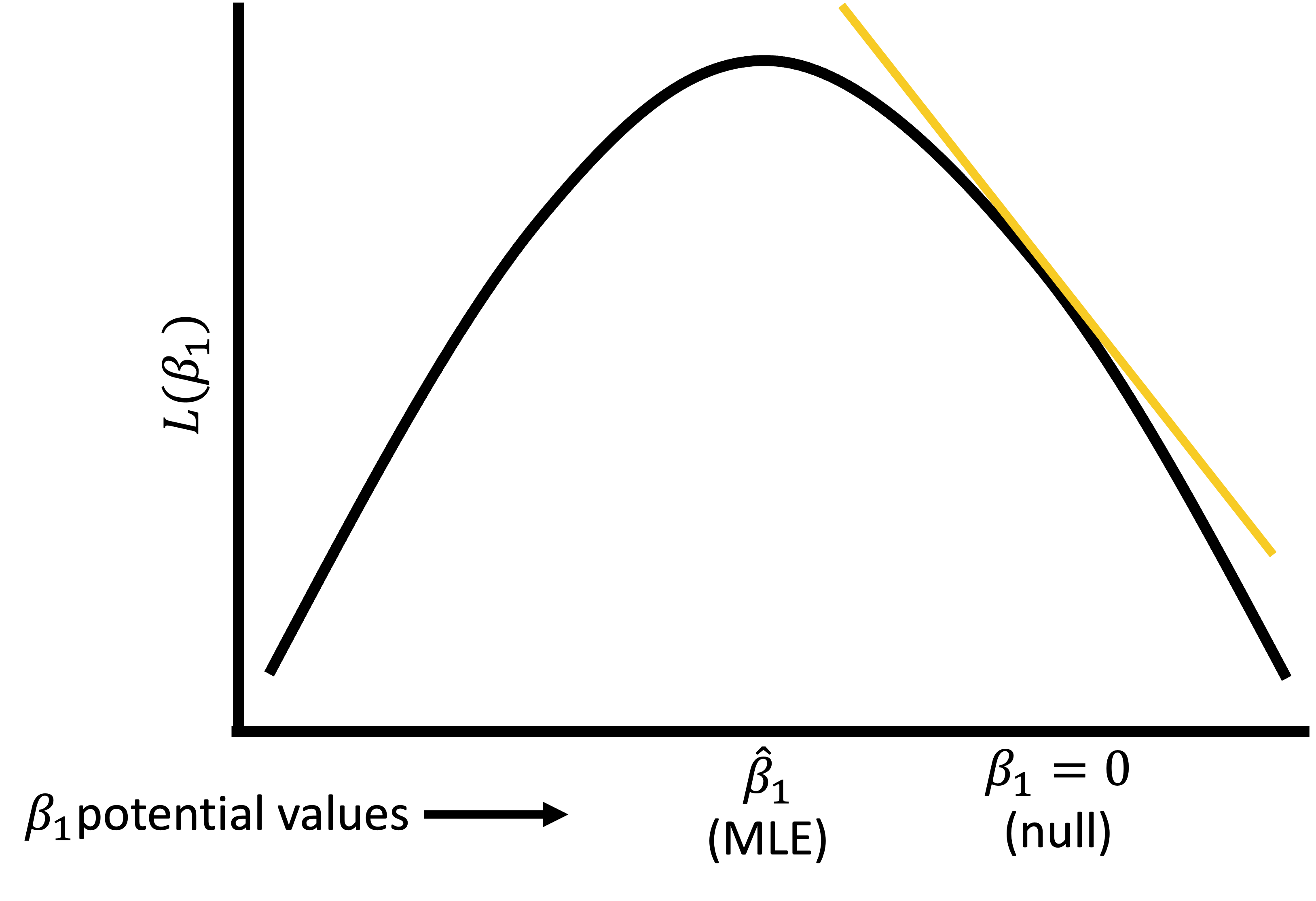
Score test
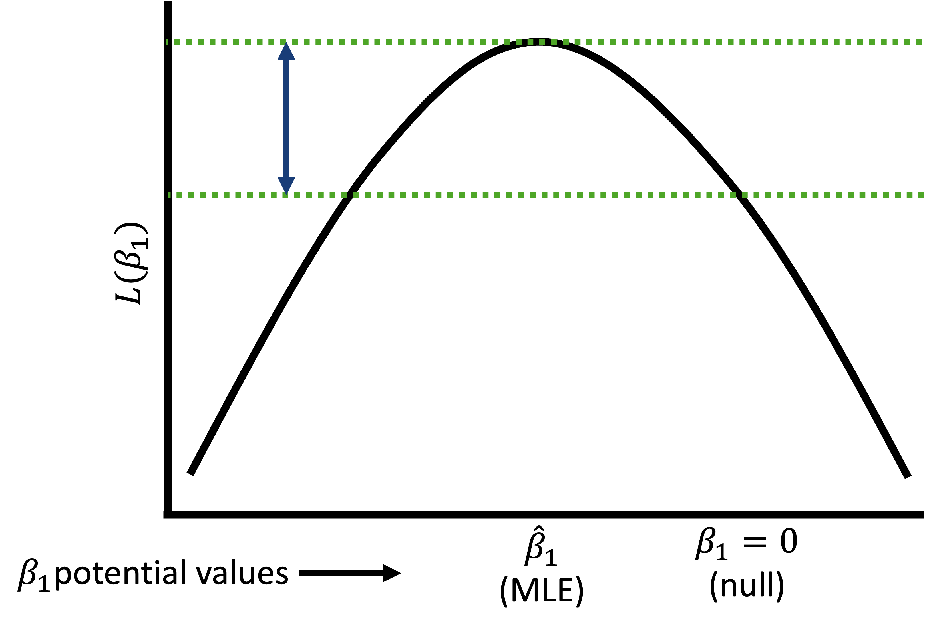
Likelihood ratio test (2/3)
- To assess the significance of a continuous/binary covariate’s coefficient in the simple logistic regression, we compare the deviance (D) with and without the covariate \[G=D\left(\text{model without } x\right)-D\left(\text{model with } x\right)\]
For a continuous or binary variable, this is equivalent to test: \(H_0: \beta_j = 0\) vs. \(H_1: \beta_j \neq 0\)
Test statistic for LRT: \[G=-2ln\left[\frac{\text{likelihood without } x}{\text{likelihood with } x}\right]=2ln\left[\frac{l\left({\hat{\beta}}_0,{\hat{\beta}}_1\right)}{l({\hat{\beta}}_0)}\right]\]

LRT: what is Deviance?
Deviance: quantifies the difference in likelihoods between a fitted and saturated model
Fitted model:
- Your proposed fitted model
Saturated model:
- A model that contains as many parameters as there are data points = perfect fit
- Basically every individual has their own covariate
- Perfect fit = maximum possible likelihood
- A model that contains as many parameters as there are data points = perfect fit
- All fitted models will have likelihood less than saturated model

LRT: what is Deviance?
The deviance is mathematically defined as: \[D=-2[L_{\text{fitted}}-L_{\text{saturated}}]\]
An alternative way to write it is: \[D=-2ln\left[\frac{\text{likelihood of the fitted model}}{\text{likelihood of the saturated model}}\right]\]
Using ‘-2’ is to make the deviance follow a chi-square distribution
Deviance to Likelihood Ratio Test
- In the LRT, we are NOT comparing the likelihood of saturated model to the fitted model
We ARE comparing the Deviance of the model with x and the model without x
- We just use the saturated model to calculate Deviance
- Both are considered fitted models with their own respective Deviance
- So our LRT is: \[G=D\left(\text{model without } x\right)-D\left(\text{model with } x\right)\]
For reference
\[ \begin{aligned} G&=D\left(\text{model without } x\right)-D\left(\text{model with }x\right) \\ G&=-2ln\left[\frac{\text{likelihood of model without } x}{\text{likelihood of saturated model}}\right]-\left(-2ln\left[\frac{\text{likelihood of model with } x}{\text{likelihood of saturated model}}\right]\right) \\ G&=-2ln\left[\frac{\text{likelihood of model without } x}{\text{likelihood of saturated model}}\times\frac{\text{likelihood of saturated model}}{\text{likelihood of model with } x}\right] \\ G&=-2ln\left[\frac{\text{likelihood of model without } x}{\text{likelihood of model with }}\right] \\ G&=2ln\left[\frac{l\left({\hat{\beta}}_0,{\hat{\beta}}_1\right)}{l({\hat{\beta}}_0)}\right] \end{aligned}\]
Likelihood ratio test (2/3)
- To assess the significance of a continuous/binary covariate’s coefficient in the simple logistic regression, we compare the deviance (D) with and without the covariate \[G=D\left(\text{model without } x\right)-D\left(\text{model with } x\right)\]
For a continuous or binary variable, this is equivalent to test: \(H_0: \beta_j = 0\) vs. \(H_1: \beta_j \neq 0\)
Test statistic for LRT: \[G=-2ln\left[\frac{\text{likelihood without } x}{\text{likelihood with } x}\right]=2ln\left[\frac{l\left({\hat{\beta}}_0,{\hat{\beta}}_1\right)}{l({\hat{\beta}}_0)}\right]\]

Likelihood ratio test
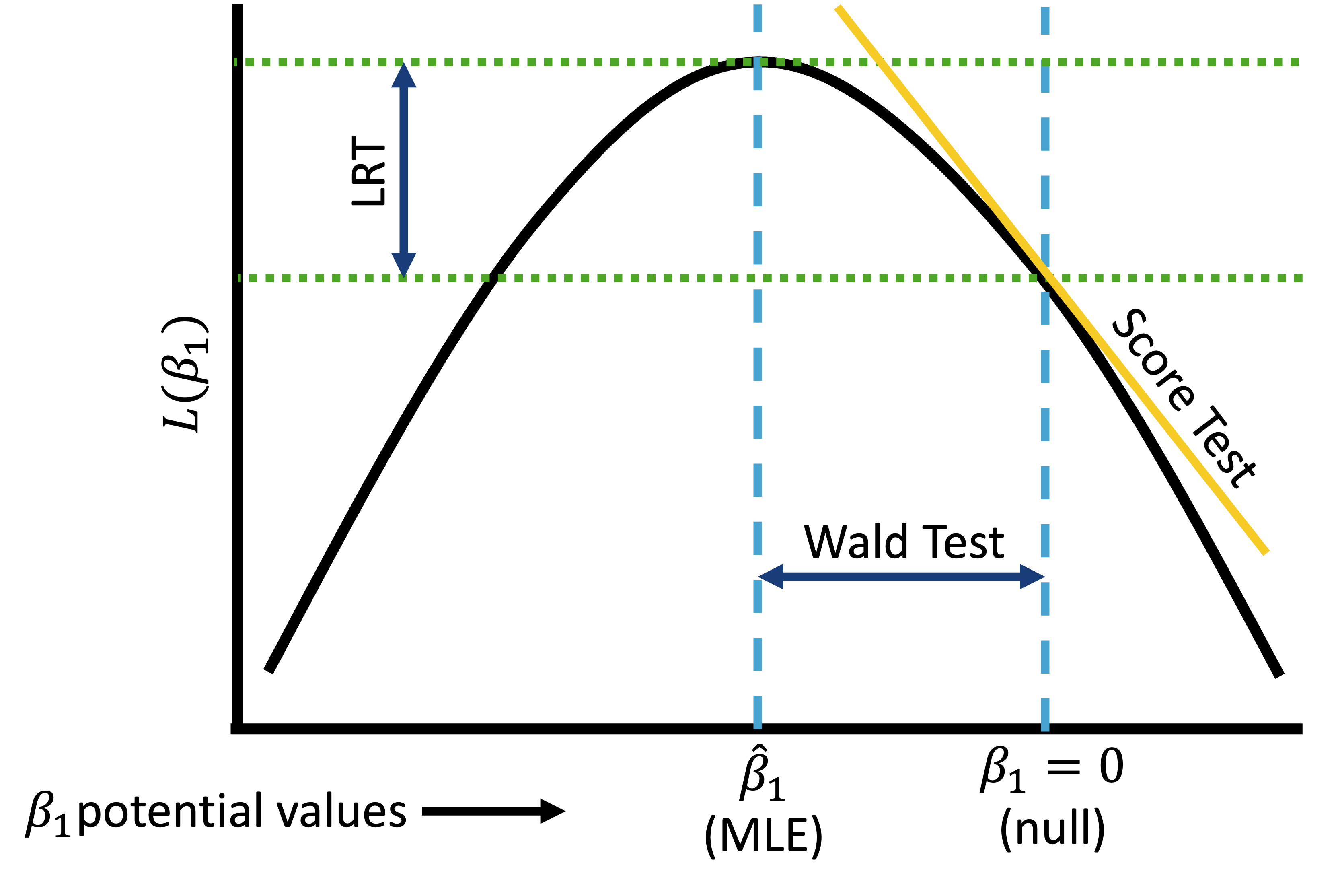
All three tests together