Lesson 7: Prediction and Visualization in Simple Logistic Regression

Nicky Wakim

2024-04-22

Learning Objectives

Make transformation between logistic regression and estimated/predicted probability.
Construct confidence interval for predicted probability.
Visualize the predicted probability (and its confidence intervals).

Recall our example: Late stage breast cancer diagnosis

Recall that we fitted a simple logistic regression for late stage breast cancer diagnosis using the predictor, age:

bc_reg = glm(Late_stage_diag ~ Age_c, data = bc, family = binomial)
tidy(bc_reg, conf.int=T) %>% gt() %>% tab_options(table.font.size = 38) %>%
  fmt_number(decimals = 3)

term	estimate	std.error	statistic	p.value	conf.low	conf.high
(Intercept)	−0.989	0.023	−42.637	0.000	−1.035	−0.944
Age_c	0.057	0.003	17.780	0.000	0.051	0.063

Fitted logistic regression model: \[\text{logit}(\widehat{\pi}(Age)) = -0.989 + 0.057 \cdot Age\]

Recall our example: Late stage breast cancer diagnosis

Fitted logistic regression model: \[\text{logit}(\widehat{\pi}(Age)) = -0.989 + 0.057 \cdot Age\]

Now we want to caclulate the predicted/estimated probability from the above fitted model
We will need to calculate the predicted probability and its confidence interval
- Then we will visualize the fitted probability

Learning Objectives

Make transformation between logistic regression and estimated/predicted probability.

Construct confidence interval for predicted probability.
Visualize the predicted probability (and its confidence intervals).

Predicted Probability

We may be interested in predicting probability of having a late stage breast cancer diagnosis for a specific age.
The predicted probability is the estimated probability of having the event for given values of covariate(s)
In simple logistic regression, the fitted model is:\[\text{logit}(\widehat{\pi}(X)) = \hat{\beta}_0 +{\hat{\beta}}_1X \]
We can convert it to the predicted probability: \[\hat{\pi}\left(X\right)=\frac{\exp({\hat{\beta}}_0+{\hat{\beta}}_1X)}{1+\exp({\hat{\beta}}_0+{\hat{\beta}}_1X)}\]
- This is an inverse logit calculation
We can calculate this using the the predict() function like in BSTA 512
- Another option: taking inverse logit of fitted values from augment() function

Reference: Inverse logit

If we have \(\text{logit}(a) = b\), then \[\begin{aligned} \text{logit}(a) & = b \\ \text{log}\left(\dfrac{a}{1-a}\right) & = b \\ \exp \left[ \text{log}\left(\dfrac{a}{1-a}\right) \right] & = \exp[b] \\ \dfrac{a}{1-a} & = \exp[b] \\ a & = \exp[b]\cdot(1-a) \\ a & = \exp[b] - a\cdot \exp[b] \\ a + a\cdot \exp[b]& = \exp[b] \\ a\cdot ( 1 + \exp[b] )& = \exp[b] \\ a& = \dfrac{\exp[b]}{1 + \exp[b]} \\ \end{aligned}\]

Learning Objectives

Make transformation between logistic regression and estimated/predicted probability.

Construct confidence interval for predicted probability.

Visualize the predicted probability (and its confidence intervals).

Confidence Interval of Predicted Probability

Not as easy to construct
I have searched around for a function that does this for us, but I cannot find one
So we have to construct the confidence interval “by hand”

There are a two ways to do this:

Construct the 95% confidence interval in the logit scale, then convert to probability scale
Use Normal approximation (if appropriate) to construct confidence interval in probability scale

Option 1: 95% confidence interval in logit scale (1/2)

Recall our our fitted simple logistic regression model with a continuous predictor \[\text{logit}(\widehat{\pi}(X)) = \widehat{\beta}_0 + \widehat{\beta}_1 \cdot X\]
We can first find the predicted \(\text{logit}(\widehat{\pi}(X))\) and then find the 95% confidence interval around it: \[\text{logit}(\widehat{\pi}(X)) \pm 1.96 \cdot SE_{\text{logit}(\widehat{\pi}(X))}\]
We’ll call this 95% CI: \[\left(\text{logit}(\widehat{\pi}(X)) - 1.96 \cdot SE_{\text{logit}(\widehat{\pi}(X))}, \ \text{logit}(\widehat{\pi}(X)) + 1.96 \cdot SE_{\text{logit}(\widehat{\pi}(X))} \right)\] \[\left(\text{logit}_{L}, \ \text{logit}_{U} \right)\]

Option 1: 95% confidence interval in logit scale (2/2)

Then we need to convert to the probability scale
To convert from \(\text{logit}(\widehat{\pi}(X))\) to \(\widehat{\pi}(X)\), we take the inverse logit
Thus, 95% CI in the probability scale is: \[\left(\dfrac{\exp\left[\text{logit}_{L}\right]}{1 + \exp\left[\text{logit}_{L}\right]}, \ \dfrac{\exp\left[\text{logit}_{U}\right]}{1 + \exp\left[\text{logit}_{U}\right]} \right)\]

Option 2: Using Normal approximation

If we meet the Normal approximation criteria, we can construct our confidence interval directly in the probability scale
- We can use the Normal approximation if:
  - \(\widehat{p}n = \widehat{\pi}(X)\cdot n > 10\) and
  - \((1-\widehat{p})n = (1-\widehat{\pi}(X))\cdot n > 10\)

We can first find the predicted \(\widehat{\pi}(X)\) and then find the 95% confidence interval around it: \[\widehat{\pi}(X) \pm 1.96 \cdot SE_{\widehat{\pi}(X)}\]

Example: Late stage breast cancer diagnosis

Predicting probability of late stage breast cancer diagnosis

For someone 50 years old, what is the predicted probability for late stage breast cancer diagnosis (with confidence intervals)?

Needed steps:

Calculate probability prediction
Check if we can use Normal approximation
Calculate confidence interval
1. Using logit scale then converting
2. Using Normal approximation
Interpret results

Example: Late stage breast cancer diagnosis

Predicting probability of late stage breast cancer diagnosis

For someone 50 years old, what is the predicted probability for late stage breast cancer diagnosis (with confidence intervals)?

Calculate probability prediction

bc_reg = glm(Late_stage_diag ~ Age_c, data = bc, family = binomial)
newdata = data.frame(Age_c = 60 - mean_age)
pred1 = predict(bc_reg, newdata = newdata, se.fit = T, type = "response")
pred1

$fit
        1 
0.2522616 

$se.fit
          1 
0.004709743 

$residual.scale
[1] 1

Example: Late stage breast cancer diagnosis

Predicting probability of late stage breast cancer diagnosis

For someone 50 years old, what is the predicted probability for late stage breast cancer diagnosis (with confidence intervals)?

Check if we can use Normal approximation

We can use the Normal approximation if: \(\widehat{p}n = \widehat{\pi}(X)\cdot n > 10\) and \((1-\widehat{p})n = (1-\widehat{\pi}(X))\cdot n > 10\).

n = nobs(bc_reg)
p = pred1$fit
n*p

       1 
2522.616

n*(1-p)

       1 
7477.384

We can use the Normal approximation!

Example: Late stage breast cancer diagnosis

Predicting probability of late stage breast cancer diagnosis

For someone 50 years old, what is the predicted probability for late stage breast cancer diagnosis (with confidence intervals)?

3a. Calculate confidence interval (Option 1: logit scale, we could skip previous step)

pred1 = predict(bc_reg, newdata = newdata, se.fit = T, type = "link")
LL_CI1 = pred1$fit - qnorm(1-0.05/2) * pred1$se.fit
UL_CI1 = pred1$fit + qnorm(1-0.05/2) * pred1$se.fit
pred_link = c(Pred = pred1$fit, LL_CI1, UL_CI1)

(exp(pred_link)/(1+exp(pred_link))) %>% round(., digits=3)

Pred.1      1      1 
 0.252  0.243  0.262

inv.logit(pred_link) %>% round(., digits=3)

Pred.1      1      1 
 0.252  0.243  0.262

Example: Late stage breast cancer diagnosis

Predicting probability of late stage breast cancer diagnosis

For someone 50 years old, what is the predicted probability for late stage breast cancer diagnosis (with confidence intervals)?

3b. Calculate confidence interval (Option 2: with Normal approximation)

pred = predict(bc_reg, newdata = newdata, se.fit = T, type = "response")

LL_CI = pred$fit - qnorm(1-0.05/2) * pred$se.fit
UL_CI = pred$fit + qnorm(1-0.05/2) * pred$se.fit

c(Pred = pred$fit, LL_CI, UL_CI) %>% round(digits=3)

Pred.1      1      1 
 0.252  0.243  0.261

Example: Late stage breast cancer diagnosis

Predicting probability of late stage breast cancer diagnosis

For someone 50 years old, what is the predicted probability for late stage breast cancer diagnosis (with confidence intervals)?

Interpret results

For someone who is 60 years old, the predicted probability of late stage breast cancer diagnosis is 0.252 (95% CI: 0.243, 0.261).

Predicted/Estimated probability

Predicted probability is NOT our predicted outcome
- We cannot interpret it as the predicted \(Y\) for individuals with certain covariate values
- Example: our predicted probability does not tell us that one individual will or will not be diagnosed with late stage breast cancer

The predicted probability is the estimate of the mean (i.e., proportion) of individuals at a certain age who are diagnosed with late stage breast cancer
We can use the predicted/estimated probability to predict the outcome

Predicted outcome

Typically, the predicted probability is the most important thing to use in a clinical setting

If you ever need to predict the outcome itself (from logistic regression with binary outcome):
- Remember that the predicted probability can be used in a Bernoulli (or Binomial with \(n=1\)) distribution to find the predicted outcome
If outcome is something like counts, then we would use a Poisson distribution

By putting it back through a Bernoulli/binomial distribution, we are re-introducing the random component of our observed outcome

set.seed(8392)
rbinom(n=1, size=1, prob = pred$fit)

[1] 0

rbinom(n=10, size=1, prob = pred$fit)

 [1] 0 0 0 0 1 0 0 0 1 0

Learning Objectives

Make transformation between logistic regression and estimated/predicted probability.
Construct confidence interval for predicted probability.

Visualize the predicted probability (and its confidence intervals).

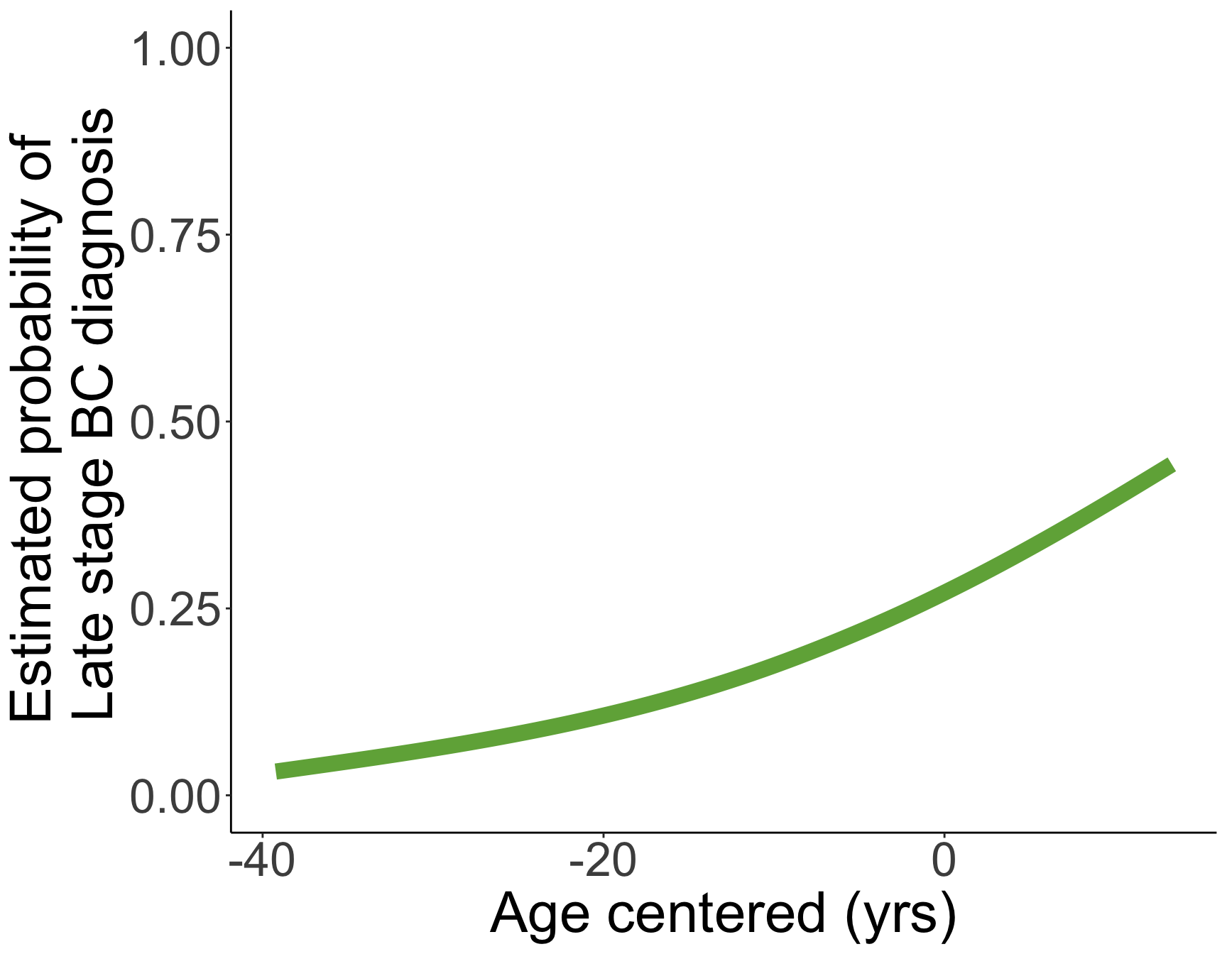
We can also make a plot of all the predicted probabilities (1/2)

bc_reg = glm(Late_stage_diag ~ Age_c, data = bc, family = binomial)
bc_aug = augment(bc_reg)

Then we plot the fitted values from the fitted model

library(boot) # for inv.logit()
prob_stage = ggplot(data = bc_aug, aes(x=Age_c, y = inv.logit(.fitted))) + 
  # geom_point(size = 4, color = "#70AD47", shape = 1) +
  geom_smooth(size = 4, color = "#70AD47") +
  labs(x = "Age centered (yrs)", 
       y = "Estimated probability of \n Late stage BC diagnosis")  + 
  theme_classic() +
  theme(axis.title = element_text(size = 30), 
        axis.text = element_text(size = 25), 
        title = element_text(size = 30)) +
  ylim(0, 1)

We can also make a plot of all the predicted probabilities (2/2)

If we are interested in seeing all the predicted probabilities across the sample’s age range
Note that the probabilities do not need to fill the full range of 0 to 1.

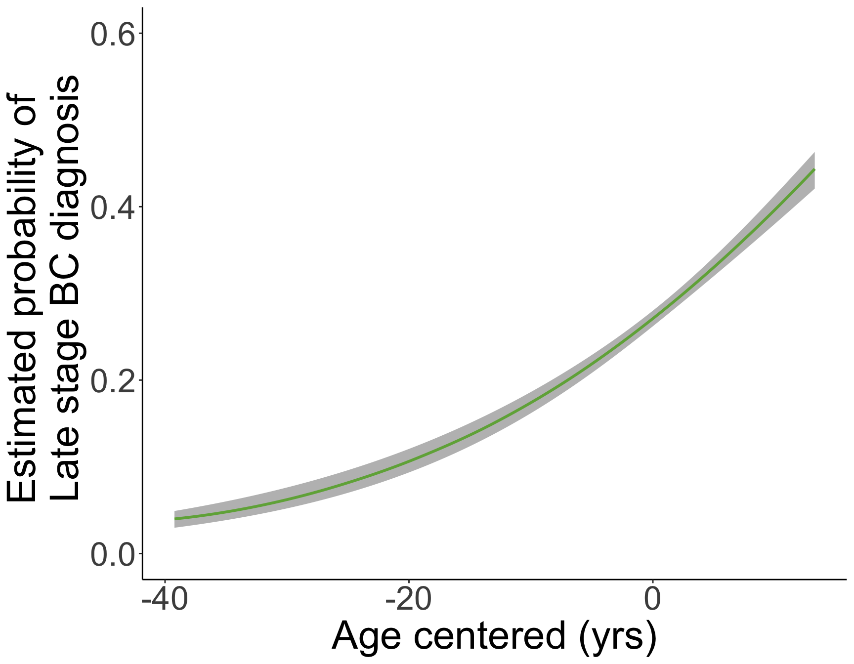
We can add the confidence intervals (1/3)

newdata2 = data.frame(Age_c = seq(min(bc$Age_c), max(bc$Age_c), by = 0.1))
pred2 = predict(bc_reg, newdata = newdata2, se.fit = T, type = "link")
LL_CI1 = pred2$fit - qnorm(1-0.05/2) * pred2$se.fit
UL_CI1 = pred2$fit + qnorm(1-0.05/2) * pred2$se.fit

with_CI = data.frame(Age_c = newdata2$Age_c, 
                     pred = inv.logit(pred2$fit), 
                     LL = inv.logit(LL_CI1), 
                     UL = inv.logit(UL_CI1))

We can add the confidence intervals (2/3)

prob_stage_CI = ggplot(data = with_CI, aes(x = Age_c)) +
  geom_ribbon(aes(ymin = LL, ymax = UL), fill = "grey") +
  geom_smooth(aes(x=Age_c, y = pred), size = 1, color = "#70AD47") +
  labs(x = "Age centered (yrs)", 
       y = "Estimated probability of \n Late stage BC diagnosis")  + 
  theme_classic() +
  theme(axis.title = element_text(size = 30), 
        axis.text = element_text(size = 25), 
        title = element_text(size = 30)) +
  ylim(0, 0.6)

We can add the confidence intervals (3/3)

Poll Everywhere Question

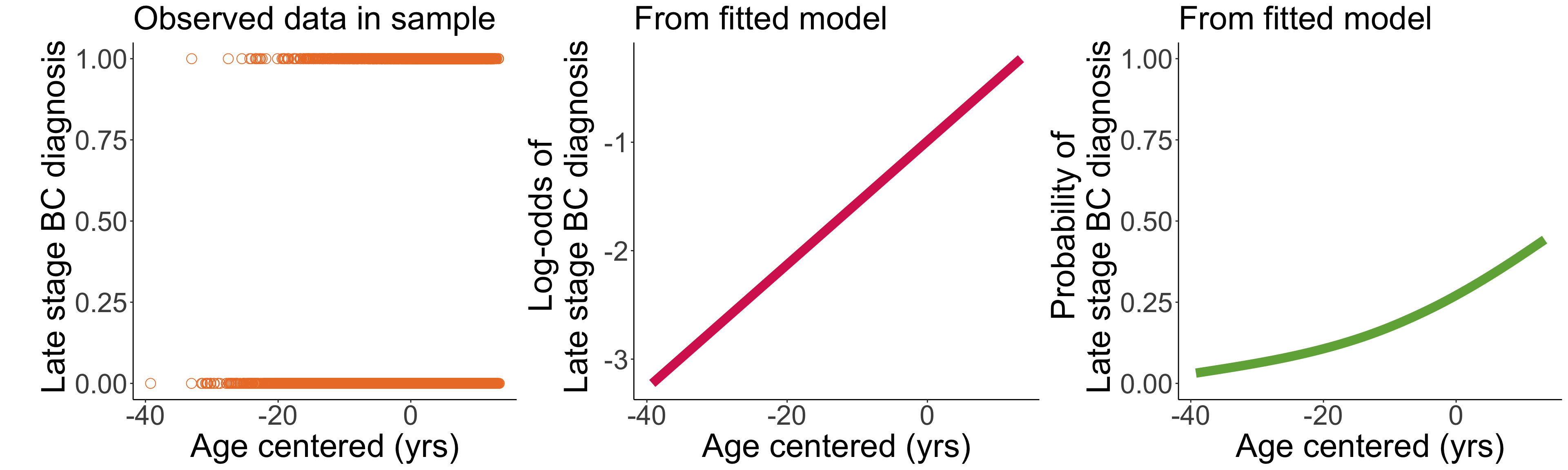
Visualization of observed outcome and fitted model

\[\text{logit}(\widehat{\pi}(Age)) = -0.989 + 0.057 \cdot Age\]

\[\widehat{\pi}(Age) = \dfrac{ \exp \left[-0.989 + 0.057 \cdot Age \right]}{1+\exp \left[-0.989 + 0.057 \cdot Age \right]}\]

Visualization of odds ratios?

We will discuss this more on Wednesday when we look at interpretations of ORs

Learning Objectives

Make transformation between logistic regression and estimated/predicted probability.
Construct confidence interval for predicted probability.
Visualize the predicted probability (and its confidence intervals).