Simple Linear Regression (SLR)

Nicky Wakim

2023-01-17

Learning Objectives

1. Identify the aims of your research and see how they align with the intended purpose of simple linear regression

2. Identify the simple linear regression model and define statistics language for key notation

3. Illustrate how ordinary least squares (OLS) finds the best model parameter estimates

4. Solve the optimal coefficient estimates for simple linear regression using OLS

5. Apply OLS in R for simple linear regression of real data

Let’s start with an example

 

Average life expectancy vs. female literacy rate

 

• Each point on the plot is for a different country

 

• \(X\) = country’s adult female literacy rate

 

• \(Y\) = country’s average life expectancy (years)

\[\widehat{\text{life expectancy}} = 50.9 + 0.232\cdot\text{female literacy rate}\]

Reference: How did I code that?

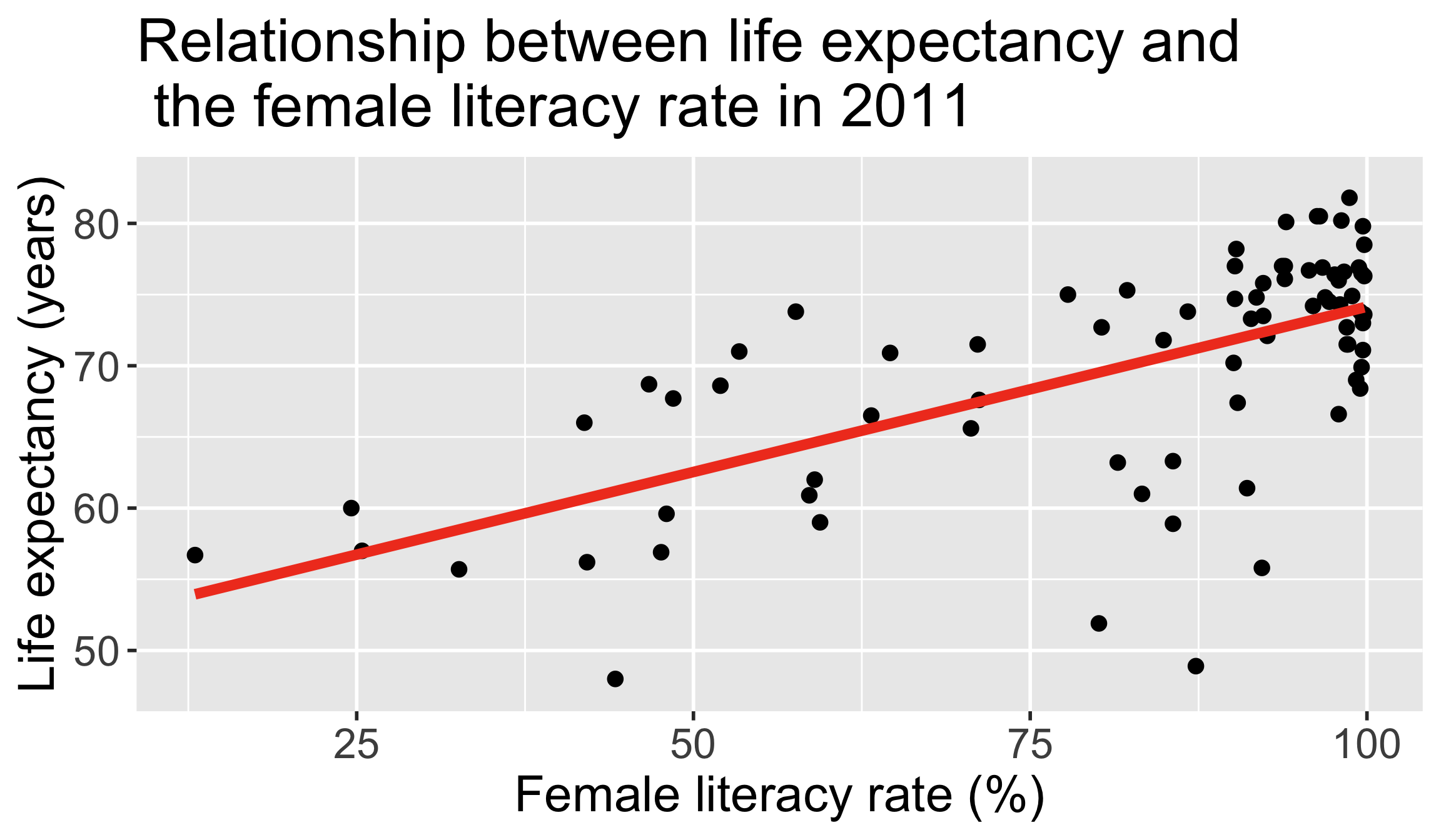
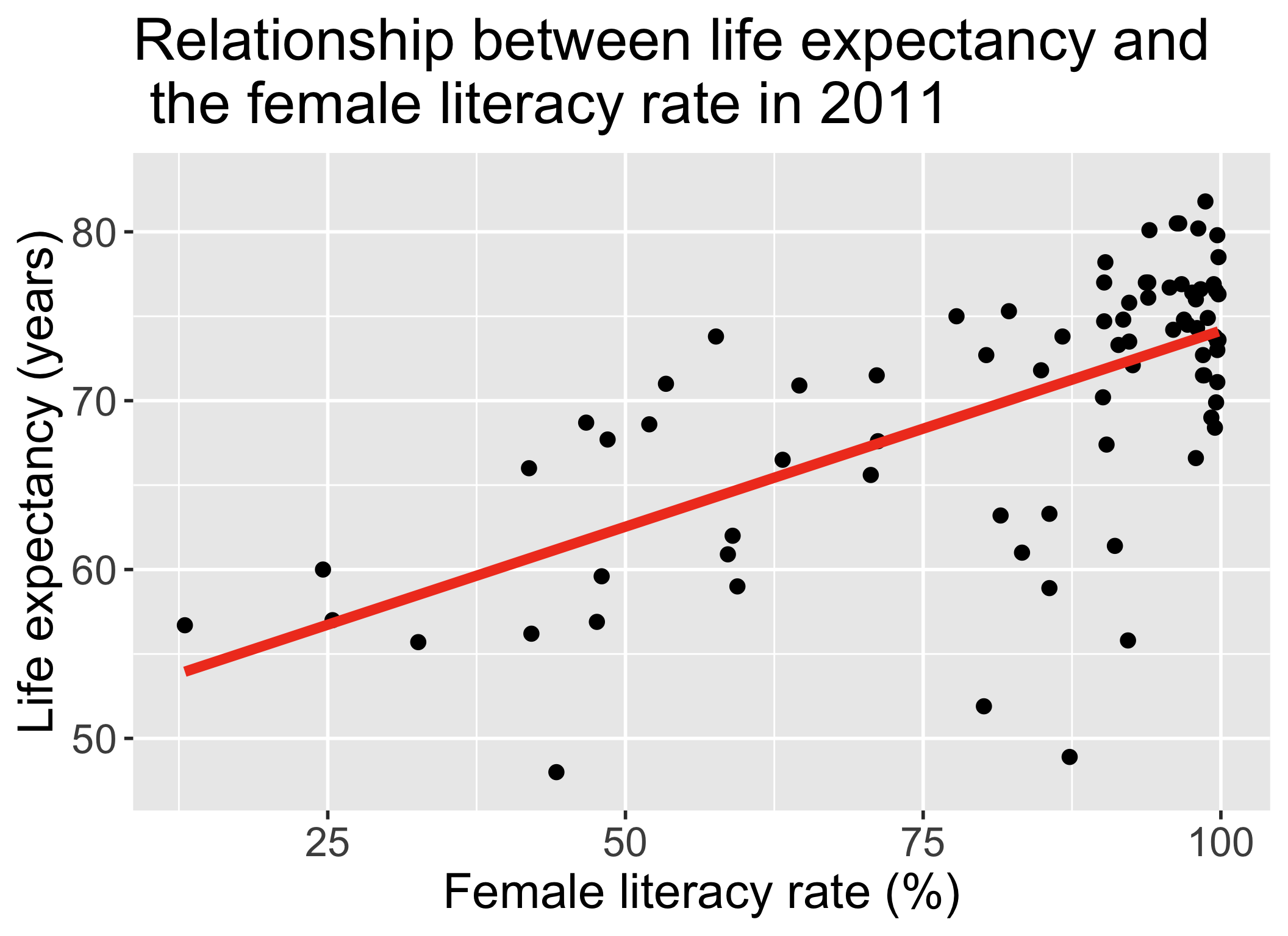
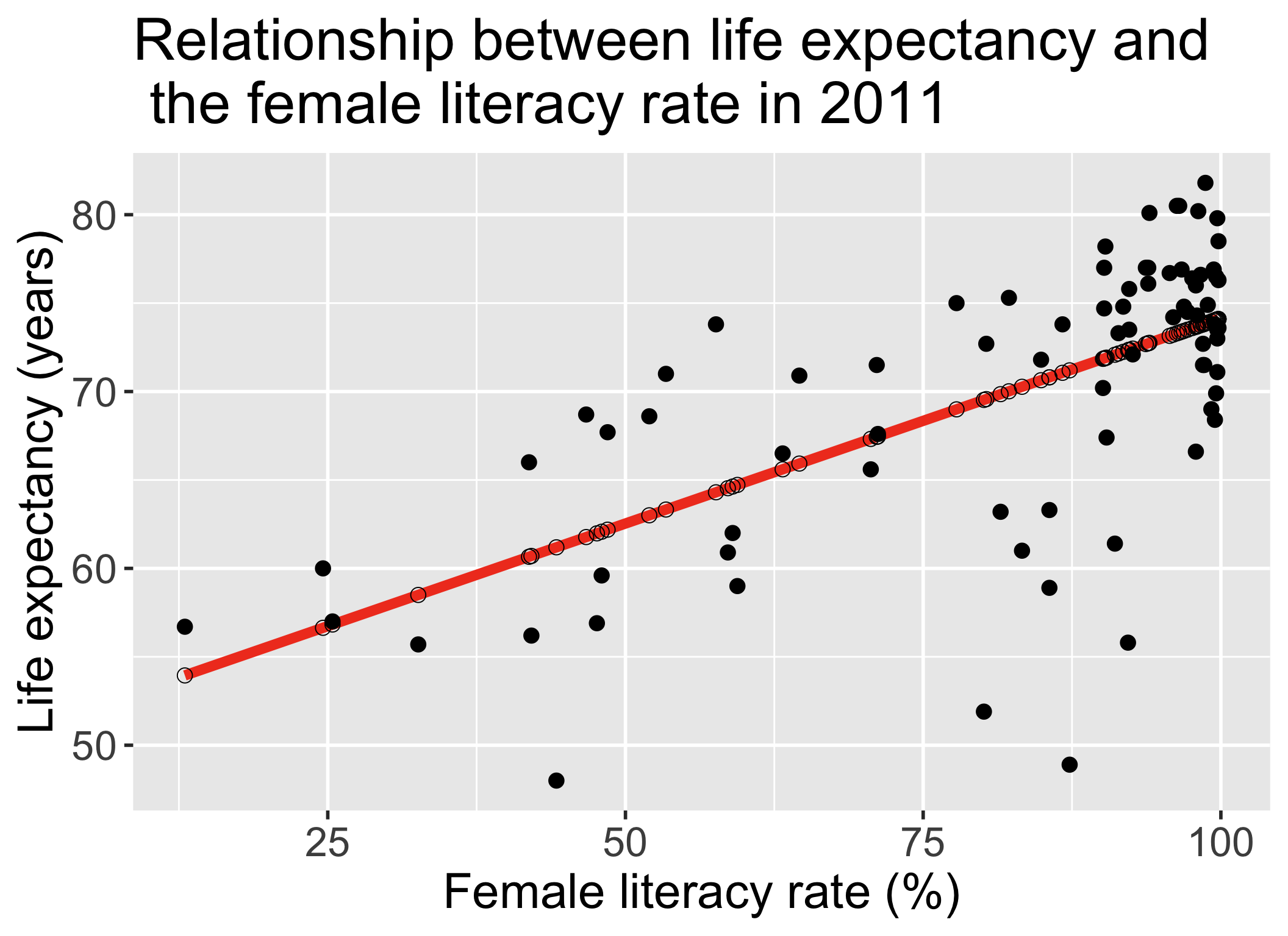
ggplot(gapm, aes(x = female_literacy_rate_2011,
                 y = life_expectancy_years_2011)) +
  geom_point(size = 4) +
  geom_smooth(method = "lm", se = FALSE, size = 3, colour="#F14124") +
  labs(x = "Female literacy rate (%)", 
       y = "Life expectancy (years)",
       title = "Relationship between life expectancy and \n the female literacy rate in 2011") +
    theme(axis.title = element_text(size = 30), 
        axis.text = element_text(size = 25), 
        title = element_text(size = 30))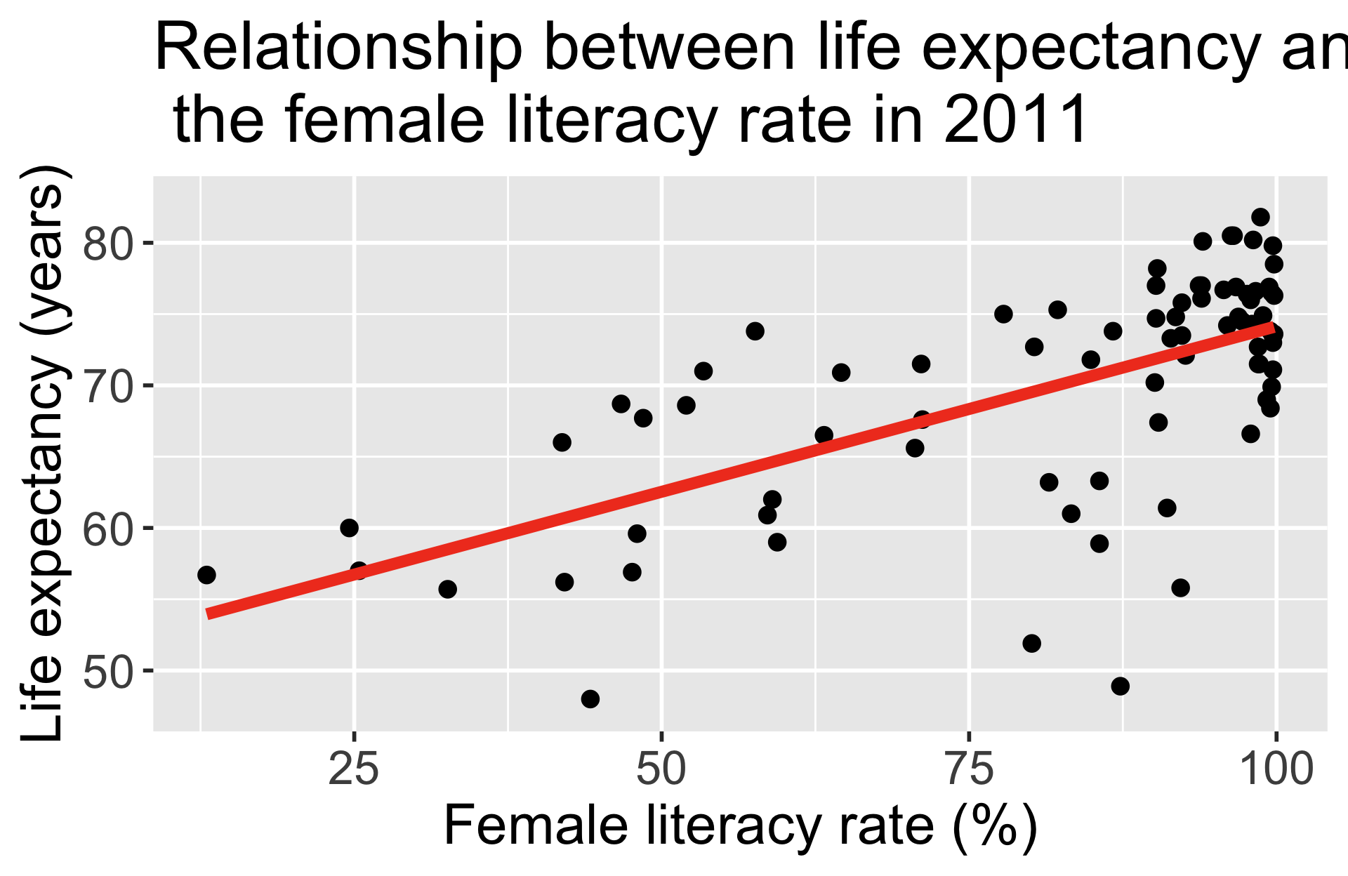

Dataset description

• Data files

  • Cleaned: lifeexp_femlit_2011.csv

  • Needs cleaning: lifeexp_femlit_water_2011.csv

• Data were downloaded from Gapminder

• 2011 is the most recent year with the most complete data

• Life expectancy = the average number of years a newborn child would live if current mortality patterns were to stay the same.

• Adult literacy rate is the percentage of people ages 15 and above who can, with understanding, read and write a short, simple statement on their everyday life.

Get to know the data (1/2)

• Load data

gapm_original <- read_csv(here::here("data", "lifeexp_femlit_water_2011.csv"))

• Glimpse of the data

glimpse(gapm_original)

Rows: 194
Columns: 5
$ country                    <chr> "Afghanistan", "Albania", "Algeria", "Andor…
$ life_expectancy_years_2011 <dbl> 56.7, 76.7, 76.7, 82.6, 60.9, 76.9, 76.0, 7…
$ female_literacy_rate_2011  <dbl> 13.0, 95.7, NA, NA, 58.6, 99.4, 97.9, 99.5,…
$ water_basic_source_2011    <dbl> 52.6, 88.1, 92.6, 100.0, 40.3, 97.0, 99.5, …
$ water_2011_quart           <chr> "Q1", "Q2", "Q2", "Q4", "Q1", "Q3", "Q4", "…

• Note the missing values for our variables of interest

Get to know the data (2/2)

• Get a sense of the summary statistics

gapm_original %>% 
  select(life_expectancy_years_2011, female_literacy_rate_2011) %>% 
  summary()

 life_expectancy_years_2011 female_literacy_rate_2011
 Min.   :47.50              Min.   :13.00            
 1st Qu.:64.30              1st Qu.:70.97            
 Median :72.70              Median :91.60            
 Mean   :70.66              Mean   :81.65            
 3rd Qu.:76.90              3rd Qu.:98.03            
 Max.   :82.90              Max.   :99.80            
 NA's   :7                  NA's   :114              

Remove missing values (1/2)

• Remove rows with missing data for life expectancy and female literacy rate

gapm <- gapm_original %>% 
  drop_na(life_expectancy_years_2011, female_literacy_rate_2011)

glimpse(gapm)

Rows: 80
Columns: 5
$ country                    <chr> "Afghanistan", "Albania", "Angola", "Antigu…
$ life_expectancy_years_2011 <dbl> 56.7, 76.7, 60.9, 76.9, 76.0, 73.8, 71.0, 7…
$ female_literacy_rate_2011  <dbl> 13.0, 95.7, 58.6, 99.4, 97.9, 99.5, 53.4, 9…
$ water_basic_source_2011    <dbl> 52.6, 88.1, 40.3, 97.0, 99.5, 97.8, 96.7, 9…
$ water_2011_quart           <chr> "Q1", "Q2", "Q1", "Q3", "Q4", "Q3", "Q3", "…

• No missing values now for our variables of interest

Remove missing values (2/2)

• And no more missing values when we look only at our two variables of interest

gapm %>% select(life_expectancy_years_2011, female_literacy_rate_2011) %>% 
  get_summary_stats()

# A tibble: 2 × 13
  variable        n   min   max median    q1    q3   iqr   mad  mean    sd    se
  <fct>       <dbl> <dbl> <dbl>  <dbl> <dbl> <dbl> <dbl> <dbl> <dbl> <dbl> <dbl>
1 life_expec…    80    48  81.8   72.4  65.9  75.8  9.95  6.30  69.9  7.95 0.889
2 female_lit…    80    13  99.8   91.6  71.0  98.0 27.0  11.4   81.7 22.0  2.45 
# ℹ 1 more variable: ci <dbl>

Note

• Removing the rows with missing data was not needed to run the regression model.
• I did this step since later we will be calculating the standard deviations of the explanatory and response variables for just the values included in the regression model. It’ll be easier to do this if we remove the missing values now.

Poll Everywhere Question 1

Learning Objectives

1. Identify the aims of your research and see how they align with the intended purpose of simple linear regression

2. Identify the simple linear regression model and define statistics language for key notation

3. Illustrate how ordinary least squares (OLS) finds the best model parameter estimates

4. Solve the optimal coefficient estimates for simple linear regression using OLS

5. Apply OLS in R for simple linear regression of real data

Questions we can ask with a simple linear regression model

• How do we…
  • calculate slope & intercept?
  • interpret slope & intercept?
  • do inference for slope & intercept?
    • CI, p-value
  • do prediction with regression line?
    • CI for prediction?
• Does the model fit the data well?
  • Should we be using a line to model the data?
• Should we add additional variables to the model?
  • multiple/multivariable regression

\[\widehat{\text{life expectancy}} = 50.9 + 0.232\cdot\text{female literacy rate}\]

Association vs. prediction

Association

• What is the association between countries’ life expectancy and female literacy rate?
• Use the slope of the line or correlation coefficient

Prediction

• What is the expected average life expectancy for a country with a specified female literacy rate?    

\[\widehat{\text{life expectancy}} = 50.9 + 0.232\cdot\text{female literacy rate}\]

Three types of study design (there are more)

Experiment

• Observational units are randomly assigned to important predictor levels

  • Random assignment controls for confounding variables (age, gender, race, etc.)

  • “gold standard” for determining causality

  • Observational unit is often at the participant-level

Quasi-experiment

• Participants are assigned to intervention levels without randomization

• Not common study design

Observational

• No randomization or assignment of intervention conditions

• In general cannot infer causality

  • However, there are casual inference methods…

Let’s revisit the regression analysis process

   

Model Selection

• Building a model

• Prediction vs interpretation

• Comparing models

Model Fitting

• Parameter estimation

• Interpret model parameters

• Hypothesis tests for coefficients

• Categorical covariates

• Interactions

Model Evaluation

• Evaluation of full and reduced models
• Testing model assumptions
• Residuals
• Transformations
• Influential points
• Multicollinearity

Poll Everywhere Question 2

Learning Objectives

1. Identify the aims of your research and see how they align with the intended purpose of simple linear regression

2. Identify the simple linear regression model and define statistics language for key notation

3. Illustrate how ordinary least squares (OLS) finds the best model parameter estimates

4. Solve the optimal coefficient estimates for simple linear regression using OLS

5. Apply OLS in R for simple linear regression of real data

Simple Linear Regression Model

The (population) regression model is denoted by:

 

\[Y = \beta_0 + \beta_1X + \epsilon\]

 

Observable sample data

• \(Y\) is our dependent variable

  • Aka outcome or response variable

• \(X\) is our independent variable

  • Aka predictor, regressor, exposure variable

Unobservable population parameters

• \(\beta_0\) and \(\beta_1\) are unknown population parameters

• \(\epsilon\) (epsilon) is the error about the line

  • It is assumed to be a random variable with a…

    • Normal distribution with mean 0 and constant variance \(\sigma^2\)

    • i.e. \(\epsilon \sim N(0, \sigma^2)\)

Simple Linear Regression Model (another way to view components)

The (population) regression model is denoted by:

 

\[Y = \beta_0 + \beta_1X + \epsilon\]

 

Components

\(Y\)	response, outcome, dependent variable
\(\beta_0\)	intercept
\(\beta_1\)	slope
\(X\)	predictor, covariate, independent variable
\(\epsilon\)	residuals, error term

If the population parameters are unobservable, how did we get the line for life expectancy?

 

Note: the population model is the true, underlying model that we are trying to estimate using our sample data

• Our goal in simple linear regression is to estimate \(\beta_0\) and \(\beta_1\)

Poll Everywhere Question 3

Okay, so how do we estimate the regression line?

 

At this point, we are going to move over to an R shiny app that I made.

 

Let’s see if we can eyeball the best-fit line!

Regression line = best-fit line

\[\widehat{Y} = \widehat{\beta}_0 + \widehat{\beta}_1 X \]

• \(\widehat{Y}\) is the predicted outcome for a specific value of \(X\)
• \(\widehat{\beta}_0\) is the intercept of the best-fit line
• \(\widehat{\beta}_1\) is the slope of the best-fit line, i.e., the increase in \(\widehat{Y}\) for every increase of one (unit increase) in \(X\)
  • slope = rise over run

Simple Linear Regression Model

Population regression model

\[Y = \beta_0 + \beta_1X + \epsilon\]

 

Components

\(Y\)	response, outcome, dependent variable
\(\beta_0\)	intercept
\(\beta_1\)	slope
\(X\)	predictor, covariate, independent variable
\(\epsilon\)	residuals, error term

Estimated regression line

\[\widehat{Y} = \widehat{\beta}_0 + \widehat{\beta}_1X\]

 

Components

\(\widehat{Y}\)	estimated expected response given predictor \(X\)
\(\widehat{\beta}_0\)	estimated intercept
\(\widehat{\beta}_1\)	estimated slope
\(X\)	predictor, covariate, independent variable

We get it, Nicky! How do we estimate the regression line?

First let’s take a break!!

Learning Objectives

1. Identify the aims of your research and see how they align with the intended purpose of simple linear regression

2. Identify the simple linear regression model and define statistics language for key notation

3. Illustrate how ordinary least squares (OLS) finds the best model parameter estimates

4. Solve the optimal coefficient estimates for simple linear regression using OLS

5. Apply OLS in R for simple linear regression of real data

It all starts with a residual…

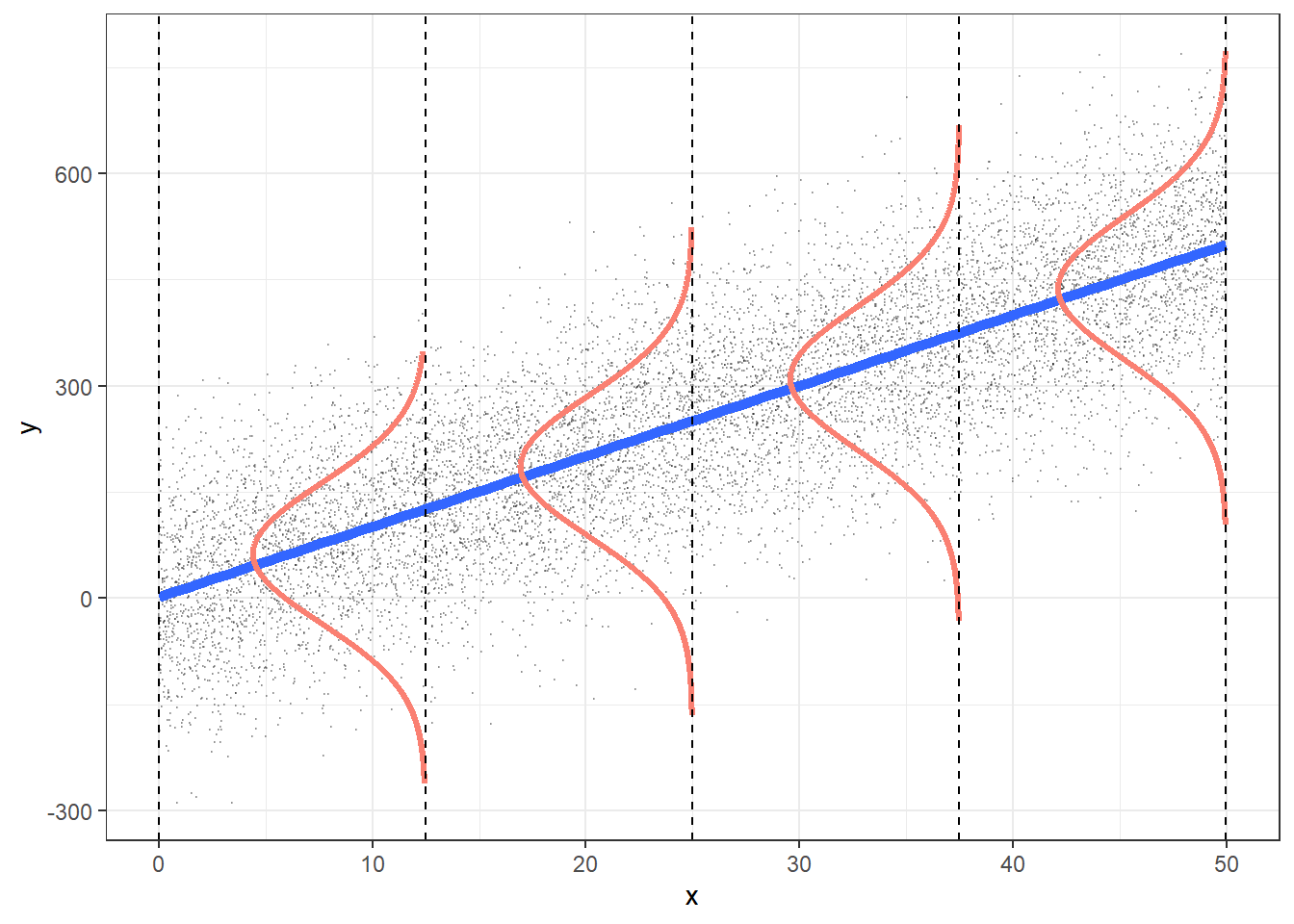
• Recall, one characteristic of our population model was that the residuals, \(\epsilon\), were Normally distributed: \(\epsilon \sim N(0, \sigma^2)\)

• In our population regression model, we had: \[Y = \beta_0 + \beta_1X + \epsilon\]

• We can also take the average (expected) value of the population model

• We take the expected value of both sides and get:

\[\begin{aligned} E[Y] & = E[\beta_0 + \beta_1X + \epsilon] \\ E[Y] & = E[\beta_0] + E[\beta_1X] + E[\epsilon] \\ E[Y] & = \beta_0 + \beta_1X + E[\epsilon] \\ E[Y|X] & = \beta_0 + \beta_1X \\ \end{aligned}\]

• We call \(E[Y|X]\) the expected value of \(Y\) given \(X\)

So now we have two representations of our population model

With observed \(Y\) values and residuals:

\[Y = \beta_0 + \beta_1X + \epsilon\]

With the population expected value of \(Y\) given \(X\):

\[E[Y|X] = \beta_0 + \beta_1X\]

Using the two forms of the model, we can figure out a formula for our residuals:

\[\begin{aligned} Y & = (\beta_0 + \beta_1X) + \epsilon \\ Y & = E[Y|X] + \epsilon \\ Y - E[Y|X] & = \epsilon \\ \epsilon & = Y - E[Y|X] \end{aligned}\]

And so we have our true, population model, residuals!

This is an important fact! For the population model, the residuals: \(\epsilon = Y - E[Y|X]\)

Back to our estimated model

We have the same two representations of our estimated/fitted model:

With observed values:

\[Y = \widehat{\beta}_0 + \widehat{\beta}_1X + \widehat{\epsilon}\]

With the estimated expected value of \(Y\) given \(X\):

\[\begin{aligned} \widehat{E}[Y|X] & = \widehat{\beta}_0 + \widehat{\beta}_1X \\ \widehat{E[Y|X]} & = \widehat{\beta}_0 + \widehat{\beta}_1X \\ \widehat{Y} & = \widehat{\beta}_0 + \widehat{\beta}_1X \\ \end{aligned}\]

Using the two forms of the model, we can figure out a formula for our estimated residuals:

\[\begin{aligned} Y & = (\widehat{\beta}_0 + \widehat{\beta}_1X) + \widehat\epsilon \\ Y & = \widehat{Y} + \widehat\epsilon \\ \widehat\epsilon & = Y - \widehat{Y} \end{aligned}\]

This is an important fact! For the estimated/fitted model, the residuals: \(\widehat\epsilon = Y - \widehat{Y}\)

Individual \(i\) residuals in the estimated/fitted model

• Observed values for each individual \(i\): \(Y_i\)
  • Value in the dataset for individual \(i\)
• Fitted value for each individual \(i\): \(\widehat{Y}_i\)
  • Value that falls on the best-fit line for a specific \(X_i\)
  • If two individuals have the same \(X_i\), then they have the same \(\widehat{Y}_i\)

Individual \(i\) residuals in the estimated/fitted model

• Observed values for each individual \(i\): \(Y_i\)

  • Value in the dataset for individual \(i\)

• Fitted value for each individual \(i\): \(\widehat{Y}_i\)

  • Value that falls on the best-fit line for a specific \(X_i\)
  • If two individuals have the same \(X_i\), then they have the same \(\widehat{Y}_i\)

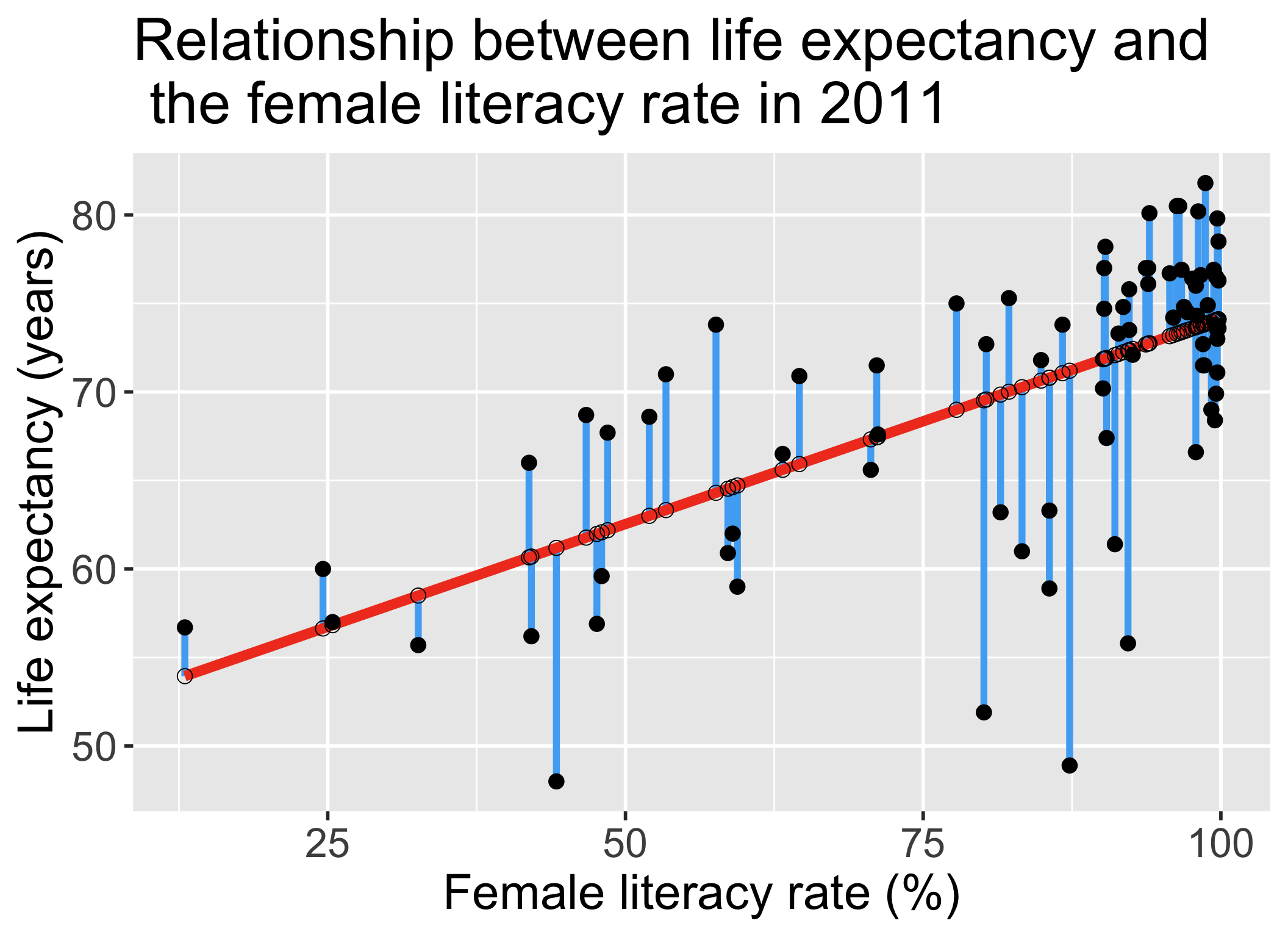
• Residual for each individual: \(\widehat\epsilon_i = Y_i - \widehat{Y}_i\)

  • Difference between the observed and fitted value

Poll Everywhere Question 4

So what do we do with the residuals?

• We want to minimize the residuals

  • Aka minimize the difference between the observed \(Y\) value and the estimated expected response given the predictor ( \(\widehat{E}[Y|X]\) )

• We can use ordinary least squares (OLS) to do this in linear regression!

• Idea behind this: reduce the total error between the fitted line and the observed point (error between is called residuals)

  • Vague use of total error: more precisely, we want to reduce the sum of squared errors
  • Think back to my R Shiny app!
  • We need to mathematically define this!

 

 

• Note: there are other ways to estimate the best-fit line!!

  • Example: Maximum likelihood estimation

Learning Objectives

1. Identify the aims of your research and see how they align with the intended purpose of simple linear regression

2. Identify the simple linear regression model and define statistics language for key notation

3. Illustrate how ordinary least squares (OLS) finds the best model parameter estimates

4. Solve the optimal coefficient estimates for simple linear regression using OLS

5. Apply OLS in R for simple linear regression of real data

Setting up for ordinary least squares

• Sum of Squared Errors (SSE)

\[ \begin{aligned} SSE & = \displaystyle\sum^n_{i=1} \widehat\epsilon_i^2 \\ SSE & = \displaystyle\sum^n_{i=1} (Y_i - \widehat{Y}_i)^2 \\ SSE & = \displaystyle\sum^n_{i=1} (Y_i - (\widehat{\beta}_0+\widehat{\beta}_1X_i))^2 \\ SSE & = \displaystyle\sum^n_{i=1} (Y_i - \widehat{\beta}_0-\widehat{\beta}_1X_i)^2 \end{aligned}\]

Things to use

• \(\widehat\epsilon_i = Y_i - \widehat{Y}_i\)

• \(\widehat{Y}_i = \widehat\beta_0 + \widehat\beta_1X_i\)

Then we want to find the estimated coefficient values that minimize the SSE!

Steps to estimate coefficients using OLS

1. Set up SSE (previous slide)

2. Minimize SSE with respect to coefficient estimates

   • Need to solve a system of equations

3. Compute derivative of SSE wrt \(\widehat\beta_0\)

4. Set derivative of SSE wrt \(\widehat\beta_0 = 0\)

5. Compute derivative of SSE wrt \(\widehat\beta_1\)

6. Set derivative of SSE wrt \(\widehat\beta_1 = 0\)

7. Substitute \(\widehat\beta_1\) back into \(\widehat\beta_0\)

2. Minimize SSE with respect to coefficients

• Want to minimize with respect to (wrt) the potential coefficient estimates ( \(\widehat\beta_0\) and \(\widehat\beta_1\))

• Take derivative of SSE wrt \(\widehat\beta_0\) and \(\widehat\beta_1\) and set equal to zero to find minimum SSE

\[ \dfrac{\partial SSE}{\partial \widehat\beta_0} = 0 \text{ and } \dfrac{\partial SSE}{\partial \widehat\beta_1} = 0 \]

• Solve the above system of equations in steps 3-6

3. Compute derivative of SSE wrt \(\widehat\beta_0\)

\[ SSE = \displaystyle\sum^n_{i=1} (Y_i - \widehat{\beta}_0-\widehat{\beta}_1X_i)^2 \]

\[\begin{aligned} \frac{\partial SSE}{\partial{\widehat{\beta}}_0}& =\frac{\partial\sum_{i=1}^{n}\left(Y_i-{\widehat{\beta}}_0-{\widehat{\beta}}_1X_i\right)^2}{\partial{\widehat{\beta}}_0}= \sum_{i=1}^{n}\frac{{\partial\left(Y_i-{\widehat{\beta}}_0-{\widehat{\beta}}_1X_i\right)}^2}{\partial{\widehat{\beta}}_0} \\ & =\sum_{i=1}^{n}{2\left(Y_i-{\widehat{\beta}}_0-{\widehat{\beta}}_1X_i\right)\left(-1\right)}=\sum_{i=1}^{n}{-2\left(Y_i-{\widehat{\beta}}_0-{\widehat{\beta}}_1X_i\right)} \\ \frac{\partial SSE}{\partial{\widehat{\beta}}_0} & = -2\sum_{i=1}^{n}\left(Y_i-{\widehat{\beta}}_0-{\widehat{\beta}}_1X_i\right) \end{aligned}\]

Things to use

• Derivative rule: derivative of sum is sum of derivative

• Derivative rule: chain rule

4. Set derivative of SSE wrt \(\widehat\beta_0 = 0\)

\[\begin{aligned} \frac{\partial SSE}{\partial{\widehat{\beta}}_0} & =0 \\ -2\sum_{i=1}^{n}\left(Y_i-{\widehat{\beta}}_0-{\widehat{\beta}}_1X_i\right) & =0 \\ \sum_{i=1}^{n}\left(Y_i-{\widehat{\beta}}_0-{\widehat{\beta}}_1X_i\right) & =0 \\ \sum_{i=1}^{n}Y_i-n{\widehat{\beta}}_0-{\widehat{\beta}}_1\sum_{i=1}^{n}X_i & =0 \\ \frac{1}{n}\sum_{i=1}^{n}Y_i-{\widehat{\beta}}_0-{\widehat{\beta}}_1\frac{1}{n}\sum_{i=1}^{n}X_i & =0 \\ \overline{Y}-{\widehat{\beta}}_0-{\widehat{\beta}}_1\overline{X} & =0 \\ {\widehat{\beta}}_0 & =\overline{Y}-{\widehat{\beta}}_1\overline{X} \end{aligned}\]

Things to use

• \(\overline{Y}=\frac{1}{n}\sum_{i=1}^{n}Y_i\)
• \(\overline{X}=\frac{1}{n}\sum_{i=1}^{n}X_i\)

5. Compute derivative of SSE wrt \(\widehat\beta_1\)

\[ SSE = \displaystyle\sum^n_{i=1} (Y_i - \widehat{\beta}_0-\widehat{\beta}_1X_i)^2 \]

\[\begin{aligned} \frac{\partial SSE}{\partial{\widehat{\beta}}_1}& =\frac{\partial\sum_{i=1}^{n}{(Y_i-{\widehat{\beta}}_0-{\widehat{\beta}}_1X_i)}^2}{\partial{\widehat{\beta}}_1}=\sum_{i=1}^{n}\frac{{\partial(Y_i-{\widehat{\beta}}_0-{\widehat{\beta}}_1X_i)}^2}{\partial{\widehat{\beta}}_1} \\ &=\sum_{i=1}^{n}{2\left(Y_i-{\widehat{\beta}}_0-{\widehat{\beta}}_1X_i\right)(-X_i)}=\sum_{i=1}^{n}{-2X_i\left(Y_i-{\widehat{\beta}}_0-{\widehat{\beta}}_1X_i\right)} \\ &=-2\sum_{i=1}^{n}{X_i\left(Y_i-{\widehat{\beta}}_0-{\widehat{\beta}}_1X_i\right)} \end{aligned}\]

Things to use

• Derivative rule: derivative of sum is sum of derivative

• Derivative rule: chain rule

6. Set derivative of SSE wrt \(\widehat\beta_1 = 0\)

\[\begin{aligned} \frac{\partial SSE}{\partial{\widehat{\beta}}_1} & =0 \\ \sum_{i=1}^{n}\left({X_iY}_i-{\widehat{\beta}}_0X_i-{\widehat{\beta}}_1{X_i}^2\right)&=0 \\ \sum_{i=1}^{n}{X_iY_i}-\sum_{i=1}^{n}{X_i{\widehat{\beta}}_0}-\sum_{i=1}^{n}{{X_i}^2{\widehat{\beta}}_1}&=0 \\ \sum_{i=1}^{n}{X_iY_i}-\sum_{i=1}^{n}{X_i\left(\overline{Y}-{\widehat{\beta}}_1\overline{X}\right)}-\sum_{i=1}^{n}{{X_i}^2{\widehat{\beta}}_1} &=0 \\ \sum_{i=1}^{n}{X_iY_i}-\sum_{i=1}^{n}{X_i\overline{Y}}+\sum_{i=1}^{n}{{\widehat{\beta}}_1X_i\overline{X}}-\sum_{i=1}^{n}{{X_i}^2{\widehat{\beta}}_1} &=0 \\ \sum_{i=1}^{n}{X_i(Y_i-\overline{Y})}+\sum_{i=1}^{n}{({\widehat{\beta}}_1X_i\overline{X}}-{X_i}^2{\widehat{\beta}}_1) &=0 \\ \sum_{i=1}^{n}{X_i(Y_i-\overline{Y})}+{\widehat{\beta}}_1\sum_{i=1}^{n}{X_i(\overline{X}}-X_i) &=0 \\ \end{aligned}\]

Things to use

• \({\widehat{\beta}}_0=\overline{Y}-{\widehat{\beta}}_1\overline{X}\)
• \(\overline{Y}=\frac{1}{n}\sum_{i=1}^{n}Y_i\)
• \(\overline{X}=\frac{1}{n}\sum_{i=1}^{n}X_i\)

         

 

\[{\widehat{\beta}}_1 =\frac{\sum_{i=1}^{n}{X_i(Y_i-\overline{Y})}}{\sum_{i=1}^{n}{X_i(}X_i-\overline{X})}\]

7. Substitute \(\widehat\beta_1\) back into \(\widehat\beta_0\)

Final coefficient estimates for SLR

Coefficient estimate for \(\widehat\beta_1\)

\[{\widehat{\beta}}_1 =\frac{\sum_{i=1}^{n}{X_i(Y_i-\overline{Y})}}{\sum_{i=1}^{n}{X_i(}X_i-\overline{X})}\]

Coefficient estimate for \(\widehat\beta_0\)

\[\begin{aligned} {\widehat{\beta}}_0 & =\overline{Y}-{\widehat{\beta}}_1\overline{X} \\ {\widehat{\beta}}_0 & = \overline{Y} - \frac{\sum_{i=1}^{n}{X_i(Y_i-\overline{Y})}}{\sum_{i=1}^{n}{X_i(}X_i-\overline{X})} \overline{X} \\ \end{aligned}\]

Poll Everywhere Question 5

Do I need to do all that work every time??

Regression in R: lm()

• Let’s discuss the syntax of this function

model1 <- lm(life_expectancy_years_2011 ~ female_literacy_rate_2011,
                 data = gapm)

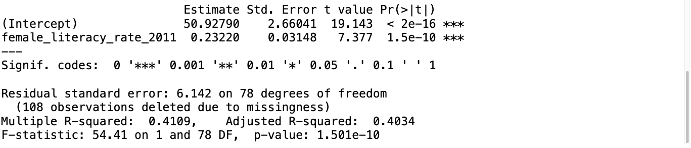
Regression in R: lm() + summary()

model1 <- lm(life_expectancy_years_2011 ~ female_literacy_rate_2011,
                 data = gapm)
summary(model1)

Call:
lm(formula = life_expectancy_years_2011 ~ female_literacy_rate_2011, 
    data = gapm)

Residuals:
    Min      1Q  Median      3Q     Max 
-22.299  -2.670   1.145   4.114   9.498 

Coefficients:
                          Estimate Std. Error t value Pr(>|t|)    
(Intercept)               50.92790    2.66041  19.143  < 2e-16 ***
female_literacy_rate_2011  0.23220    0.03148   7.377  1.5e-10 ***
---
Signif. codes:  0 '***' 0.001 '**' 0.01 '*' 0.05 '.' 0.1 ' ' 1

Residual standard error: 6.142 on 78 degrees of freedom
  (108 observations deleted due to missingness)
Multiple R-squared:  0.4109,    Adjusted R-squared:  0.4034 
F-statistic: 54.41 on 1 and 78 DF,  p-value: 1.501e-10

Regression in R: lm() + tidy()

 

tidy(model1) %>% 
  gt() %>% 
  tab_options(table.font.size = 45)

term	estimate	std.error	statistic	p.value
(Intercept)	50.9278981	2.66040695	19.142898	3.325312e-31
female_literacy_rate_2011	0.2321951	0.03147744	7.376557	1.501286e-10

 

• Regression equation for our model (which we saw a looong time ago):

\[\widehat{\text{life expectancy}} = 50.9 + 0.232\cdot\text{female literacy rate}\]

How do we interpret the coefficients?

\[\widehat{\text{life expectancy}} = 50.9 + 0.232\cdot\text{female literacy rate}\]

• Intercept
  • The expected outcome for the \(Y\)-variable when the \(X\)-variable is 0
  • Example: The expected/average life expectancy is 50.9 years for a country with 0% female literacy.
• Slope

  • For every increase of 1 unit in the \(X\)-variable, there is an expected increase of, on average, \(\widehat\beta_1\) units in the \(Y\)-variable.

  • We only say that there is an expected increase and not necessarily a causal increase.

  • Example: For every 1 percent increase in the female literacy rate, the expected/average life expectancy increases, on average, 0.232 years.

Next time

• Inference of our estimated coefficients

• Inference of estimated expected \(Y\) given \(X\)

• Prediction

• Hypothesis testing!