SLR: Inference and Prediction

Nicky Wakim

2023-01-22

Learning Objectives

1. Estimate the variance of the residuals
2. Using a hypothesis test, determine if there is enough evidence that population slope \(\beta_1\) is not 0 (applies to \(\beta_0\) as well)
3. Calculate and report the estimate and confidence interval for the population slope \(\beta_1\) (applies to \(\beta_0\) as well)
4. Calculate and report the estimate and confidence interval for the expected/mean response given \(X\)

Let’s revisit the regression analysis process

Model Selection

• Building a model

• Selecting variables

• Prediction vs interpretation

• Comparing potential models

Model Fitting

• Find best fit line

• Using OLS in this class

• Parameter estimation

• Categorical covariates

• Interactions

Model Evaluation

• Evaluation of model fit
• Testing model assumptions
• Residuals
• Transformations
• Influential points
• Multicollinearity

Model Use (Inference)

• Inference for coefficients
• Hypothesis testing for coefficients

• Inference for expected \(Y\) given \(X\)
• Prediction of new \(Y\) given \(X\)

Let’s remind ourselves of the model that we fit last lesson

• We fit Gapminder data with female literacy rate as our independent variable and life expectancy as our dependent variable

• We used OLS to find the coefficient estimates of our best-fit line

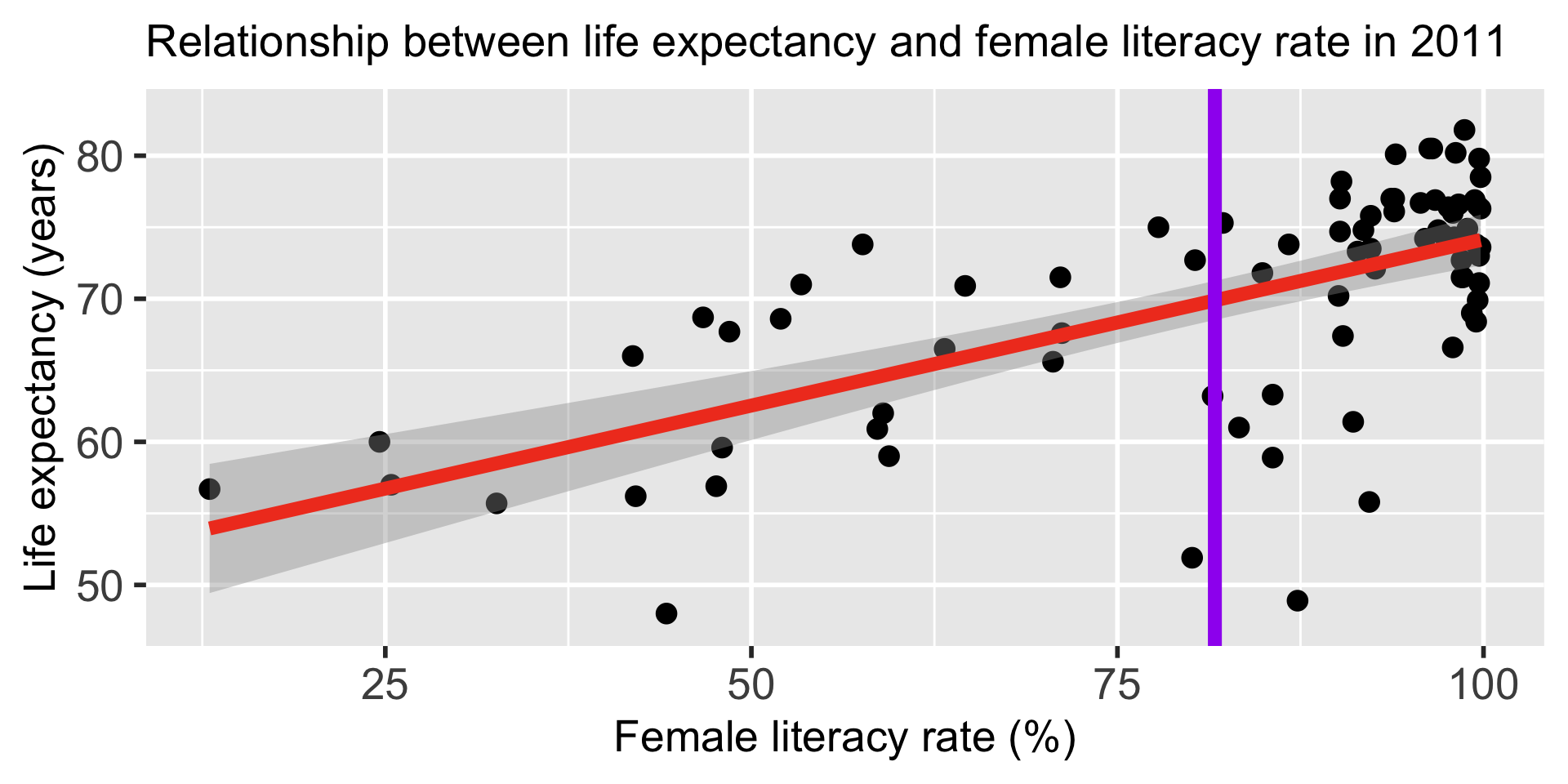
model1 <- lm(life_expectancy_years_2011 ~
               female_literacy_rate_2011,
                 data = gapm)
# Get regression table:
tidy(model1) %>% gt() %>% 
 tab_options(table.font.size = 40) %>%
 fmt_number(decimals = 2)

term	estimate	std.error	statistic	p.value
(Intercept)	50.93	2.66	19.14	0.00
female_literacy_rate_2011	0.23	0.03	7.38	0.00

\[\begin{aligned} \widehat{Y} &= \widehat\beta_0 + \widehat\beta_1 \cdot X\\ \widehat{\text{life expectancy}} &= 50.9 + 0.232 \cdot \text{female literacy rate} \end{aligned}\]

Fitted line is derived from the population SLR model

 

The (population) regression model is denoted by:

\[Y = \beta_0 + \beta_1X + \epsilon\]

• \(\beta_0\) and \(\beta_1\) are unknown population parameters

• \(\epsilon\) (epsilon) is the error about the line

  • It is assumed to be a random variable with a…

    • Normal distribution with mean 0 and constant variance \(\sigma^2\)

    • i.e. \(\epsilon \sim N(0, \sigma^2)\)

Poll Everywhere Question 1

Learning Objectives

1. Estimate the variance of the residuals

2. Using a hypothesis test, determine if there is enough evidence that population slope \(\beta_1\) is not 0 (applies to \(\beta_0\) as well)
3. Calculate and report the estimate and confidence interval for the population slope \(\beta_1\) (applies to \(\beta_0\) as well)
4. Calculate and report the estimate and confidence interval for the expected/mean response given \(X\)

\(\widehat\sigma^2\): Needed ingredient for inference

• Recall our population model residuals are distributed by \(\epsilon \sim N(0, \sigma^2)\)
  • And our estimated residuals are \(\widehat\epsilon \sim N(0, \widehat\sigma^2)\)
• Hence, the variance of the errors (residuals) is estimated by \(\widehat{\sigma}^2\)

\[\widehat{\sigma}^2 = S_{y|x}^2= \frac{1}{n-2}\sum_{i=1}^n (Y_i - \widehat{Y}_i)^2 =\frac{1}{n-2}SSE = MSE\]

\(\widehat\sigma^2\): I hope R can calculate that for me…

• The standard deviation \(\widehat{\sigma}\) is given in the R output as the Residual standard error

  • \(4^{th}\) line from the bottom in the summary() output of the model:

(m1_sum = summary(model1))

Call:
lm(formula = life_expectancy_years_2011 ~ female_literacy_rate_2011, 
    data = gapm)

Residuals:
    Min      1Q  Median      3Q     Max 
-22.299  -2.670   1.145   4.114   9.498 

Coefficients:
                          Estimate Std. Error t value Pr(>|t|)    
(Intercept)               50.92790    2.66041  19.143  < 2e-16 ***
female_literacy_rate_2011  0.23220    0.03148   7.377  1.5e-10 ***
---
Signif. codes:  0 '***' 0.001 '**' 0.01 '*' 0.05 '.' 0.1 ' ' 1

Residual standard error: 6.142 on 78 degrees of freedom
  (108 observations deleted due to missingness)
Multiple R-squared:  0.4109,    Adjusted R-squared:  0.4034 
F-statistic: 54.41 on 1 and 78 DF,  p-value: 1.501e-10

m1_sum$sigma

[1] 6.142157

# number of observations (pairs of data) used to run the model
nobs(model1) 

[1] 80

\(\widehat\sigma^2\) to SSE

• Recall how we minimized the SSE to find our line of best fit
• SSE and \(\widehat\sigma^2\) are closely related:

\[\begin{aligned} \widehat{\sigma}^2 & = \frac{1}{n-2}SSE\\ 6.142^2 & = \frac{1}{80-2}SSE\\ SSE & = 78 \cdot 6.142^2 = 2942.48 \end{aligned}\]

• 2942.48 is the smallest sums of squares of all possible regression lines through the data

Learning Objectives

1. Estimate the variance of the residuals

2. Using a hypothesis test, determine if there is enough evidence that population slope \(\beta_1\) is not 0 (applies to \(\beta_0\) as well)

3. Calculate and report the estimate and confidence interval for the population slope \(\beta_1\) (applies to \(\beta_0\) as well)

4. Calculate and report the estimate and confidence interval for the expected/mean response given \(X\)

Do we trust our estimate \(\widehat\beta_1\)?

• So far, we have shown that we think the estimate is 0.232  
• \(\widehat\beta_1\) uses our sample data to estimate the population parameter \(\beta_1\)  
• Inference helps us figure out _{mathematically} how much we trust our best-fit line  
• Are we certain that the relationship between \(X\) and \(Y\) that we estimated reflects the true, underlying relationship?

Poll Everywhere Question 2

Inference for the population slope: hypothesis test and CI

Population model

line + random “noise”

\[Y = \beta_0 + \beta_1 \cdot X + \varepsilon\] with \(\varepsilon \sim N(0,\sigma^2)\)
\(\sigma^2\) is the variance of the residuals

Sample best-fit (least-squares) line

\[\widehat{Y} = \widehat{\beta}_0 + \widehat{\beta}_1 \cdot X \]

Note: Some sources use \(b\) instead of \(\widehat{\beta}\)

 

We have two options for inference:

1. Conduct the hypothesis test

\[\begin{align} H_0 &: \beta_1 = 0\\ \text{vs. } H_A&: \beta_1 \neq 0 \end{align}\]

Note: R reports p-values for 2-sided tests

2. Construct a 95% confidence interval for the population slope \(\beta_1\)

Learning Objectives

1. Estimate the variance of the residuals

2. Using a hypothesis test, determine if there is enough evidence that population slope \(\beta_1\) is not 0 (applies to \(\beta_0\) as well)

3. Calculate and report the estimate and confidence interval for the population slope \(\beta_1\) (applies to \(\beta_0\) as well)
4. Calculate and report the estimate and confidence interval for the expected/mean response given \(X\)

Steps in hypothesis testing

General steps for hypothesis test for population slope \(\beta_1\) (t-test)

1. For today’s class, we are assuming that we have met the underlying assumptions (checked in our Model Evaluation step)

2. State the null hypothesis.

Often, we are curious if the coefficient is 0 or not:

\[\begin{align} H_0 &: \beta_1 = 0\\ \text{vs. } H_A&: \beta_1 \neq 0 \end{align}\]

3. Specify the significance level.

Often we use \(\alpha = 0.05\)

4. Specify the test statistic and its distribution under the null

The test statistic is \(t\), and follows a Student’s t-distribution.

5. Compute the value of the test statistic

The calculated test statistic for \(\widehat\beta_1\) is

\[t = \frac{ \widehat\beta_1 - \beta_1}{ \text{SE}_{\widehat\beta_1}} = \frac{ \widehat\beta_1}{ \text{SE}_{\widehat\beta_1}}\]

when we assume \(H_0: \beta_1 = 0\) is true.

6. Calculate the p-value

We are generally calculating: \(2\cdot P(T > t)\)

7. Write conclusion for hypothesis test

We (reject/fail to reject) the null hypothesis that the slope is 0 at the \(100\alpha\%\) significiance level. There is (sufficient/insufficient) evidence that there is significant association between (\(Y\)) and (\(X\)) (p-value = \(P(T > t)\)).

Standard error of fitted slope \(\widehat\beta_1\)

   

\[\text{SE}_{\widehat\beta_1} = \frac{s_{\textrm{residuals}}}{s_x\sqrt{n-1}}\]

\(\text{SE}_{\widehat\beta_1}\) is the variability of the statistic \(\widehat\beta_1\)

   

• \(s_{\textrm{residuals}}^2\) is the sd of the residuals

• \(s_x\) is the sample sd of the explanatory variable \(x\)

• \(n\) is the sample size, or the number of (complete) pairs of points

Calculating standard error for \(\widehat\beta_1\) (1/2)

• Option 1: Calculate using the formula

glance(model1)

# A tibble: 1 × 12
  r.squared adj.r.squared sigma statistic  p.value    df logLik   AIC   BIC
      <dbl>         <dbl> <dbl>     <dbl>    <dbl> <dbl>  <dbl> <dbl> <dbl>
1     0.411         0.403  6.14      54.4 1.50e-10     1  -258.  521.  529.
# ℹ 3 more variables: deviance <dbl>, df.residual <int>, nobs <int>

# standard deviation of the residuals (Residual standard error in summary() output)
(s_resid <- glance(model1)$sigma)

[1] 6.142157

# standard deviation of x's
(s_x <- sd(gapm$female_literacy_rate_2011, na.rm=T))

[1] 21.95371

# number of pairs of complete observations
(n <- nobs(model1))

[1] 80

(se_b1 <- s_resid/(s_x * sqrt(n-1))) # compare to SE in regression output

[1] 0.03147744

Calculating standard error for \(\widehat\beta_1\) (2/2)

• Option 2: Use regression table

# recall model1_b1 is regression table restricted to b1 row
model1_b1 <-tidy(model1) %>% filter(term == "female_literacy_rate_2011")
model1_b1 %>% gt() %>%
  tab_options(table.font.size = 45) %>% fmt_number(decimals = 4)

term	estimate	std.error	statistic	p.value
female_literacy_rate_2011	0.2322	0.0315	7.3766	0.0000

Some important notes

• Today we are discussing the hypothesis test for a single coefficient

 

• The test statistic for a single coefficient follows a Student’s t-distribution

   

  • It can also follow an F-distribution, but we will discuss this more with multiple linear regression and multi-level categorical covariates

 

• Single coefficient testing can be done on any coefficient, but it is most useful for continuous covariates or binary covariates

   

  • This is because testing the single coefficient will still tell us something about the overall relationship between the covariate and the outcome

   

  • We will talk more about this with multiple linear regression and multi-level categorical covariates

Poll Everywhere Question 3

Life expectancy example: hypothesis test for population slope \(\beta_1\) (1/4)

• Steps 1-4 are setting up our hypothesis test: not much change from the general steps

1. For today’s class, we are assuming that we have met the underlying assumptions (checked in our Model Evaluation step)

2. State the null hypothesis.

We are testing if the slope is 0 or not:

\[\begin{align} H_0 &: \beta_1 = 0\\ \text{vs. } H_A&: \beta_1 \neq 0 \end{align}\]

3. Specify the significance level.

Often we use \(\alpha = 0.05\)

4. Specify the test statistic and its distribution under the null

The test statistic is \(t\), and follows a Student’s t-distribution.

Life expectancy example: hypothesis test for population slope \(\beta_1\) (2/4)

5. Compute the value of the test statistic

• Option 1: Calculate the test statistic using the values in the regression table

# recall model1_b1 is regression table restricted to b1 row
model1_b1 <-tidy(model1) %>% filter(term == "female_literacy_rate_2011")
model1_b1 %>% gt() %>%
  tab_options(table.font.size = 40) %>% fmt_number(decimals = 2)

term	estimate	std.error	statistic	p.value
female_literacy_rate_2011	0.23	0.03	7.38	0.00

(TestStat_b1 <- model1_b1$estimate / model1_b1$std.error)

[1] 7.376557

• Option 2: Get the test statistic value (\(t^*\)) from R

model1_b1 %>% gt() %>%
  tab_options(table.font.size = 40) %>% fmt_number(decimals = 2)

term	estimate	std.error	statistic	p.value
female_literacy_rate_2011	0.23	0.03	7.38	0.00

Life expectancy example: hypothesis test for population slope \(\beta_1\) (3/4)

6. Calculate the p-value

• The \(p\)-value is the probability of obtaining a test statistic just as extreme or more extreme than the observed test statistic assuming the null hypothesis \(H_0\) is true

• We know the probability distribution of the test statistic (the null distribution) assuming \(H_0\) is true

• Statistical theory tells us that the test statistic \(t\) can be modeled by a \(t\)-distribution with \(df = n-2\).

  • We had 80 countries’ data, so \(n=80\)

• Option 1: Use pt() and our calculated test statistic

(pv = 2*pt(TestStat_b1, df=80-2, lower.tail=F))

[1] 1.501286e-10

• Option 2: Use the regression table output

model1_b1 %>% gt() %>%
  tab_options(table.font.size = 40)

term	estimate	std.error	statistic	p.value
female_literacy_rate_2011	0.2321951	0.03147744	7.376557	1.501286e-10

Life expectancy example: hypothesis test for population slope \(\beta_1\) (4/4)

7. Write conclusion for the hypothesis test

We reject the null hypothesis that the slope is 0 at the \(5\%\) significance level. There is sufficient evidence that there is significant association between female life expectancy and female literacy rates (p-value < 0.0001).

Note on hypothesis testing using R

• We can basically skip Step 5 if we are using the “Option 2” route

 

• In our assignments: if you use Option 2, Step 5 is optional

  • Unless I specifically ask for the test statistic!!

Life expectancy ex: hypothesis test for population intercept \(\beta_0\) (1/4)

• Steps 1-4 are setting up our hypothesis test: not much change from the general steps

1. For today’s class, we are assuming that we have met the underlying assumptions (checked in our Model Evaluation step)

2. State the null hypothesis.

We are testing if the intercept is 0 or not:

\[\begin{align} H_0 &: \beta_0 = 0\\ \text{vs. } H_A&: \beta_0 \neq 0 \end{align}\]

3. Specify the significance level

Often we use \(\alpha = 0.05\)

4. Specify the test statistic and its distribution under the null

This is the same as the slope. The test statistic is \(t\), and follows a Student’s t-distribution.

Life expectancy ex: hypothesis test for population intercept \(\beta_0\) (2/4)

5. Compute the value of the test statistic

• Option 1: Calculate the test statistic using the values in the regression table

# recall model1_b1 is regression table restricted to b1 row
model1_b0 <-tidy(model1) %>% filter(term == "(Intercept)")
model1_b0 %>% gt() %>%
  tab_options(table.font.size = 40) %>% fmt_number(decimals = 2)

term	estimate	std.error	statistic	p.value
(Intercept)	50.93	2.66	19.14	0.00

(TestStat_b0 <- model1_b0$estimate / model1_b0$std.error)

[1] 19.1429

• Option 2: Get the test statistic value (\(t^*\)) from R

model1_b0 %>% gt() %>%
  tab_options(table.font.size = 40) %>% fmt_number(decimals = 2)

term	estimate	std.error	statistic	p.value
(Intercept)	50.93	2.66	19.14	0.00

Life expectancy ex: hypothesis test for population intercept \(\beta_0\) (3/4)

6. Calculate the p-value

 

• Option 1: Use pt() and our calculated test statistic

(pv = 2*pt(TestStat_b0, df=80-2, lower.tail=F))

[1] 3.325312e-31

 

• Option 2: Use the regression table output

model1_b0 %>% gt() %>%
  tab_options(table.font.size = 40)

term	estimate	std.error	statistic	p.value
(Intercept)	50.9279	2.660407	19.1429	3.325312e-31

Life expectancy ex: hypothesis test for population intercept \(\beta_0\) (4/4)

7. Write conclusion for the hypothesis test

We reject the null hypothesis that the intercept is 0 at the \(5\%\) significance level. There is sufficient evidence that the intercept for the association between average female life expectancy and female literacy rates is different from 0 (p-value < 0.0001).

   

• Note: if we fail to reject \(H_0\), then we could decide to remove the intercept from the model to force the regression line to go through the origin (0,0) if it makes sense to do so for the application.

Learning Objectives

1. Estimate the variance of the residuals
2. Using a hypothesis test, determine if there is enough evidence that population slope \(\beta_1\) is not 0 (applies to \(\beta_0\) as well)

3. Calculate and report the estimate and confidence interval for the population slope \(\beta_1\) (applies to \(\beta_0\) as well)

4. Calculate and report the estimate and confidence interval for the expected/mean response given \(X\)

Inference for the population slope: hypothesis test and CI

Population model

line + random “noise”

\[Y = \beta_0 + \beta_1 \cdot X + \varepsilon\] with \(\varepsilon \sim N(0,\sigma^2)\)
\(\sigma^2\) is the variance of the residuals

Sample best-fit (least-squares) line

\[\widehat{Y} = \widehat{\beta}_0 + \widehat{\beta}_1 \cdot X \]

Note: Some sources use \(b\) instead of \(\widehat{\beta}\)

 

We have two options for inference:

1. Conduct the hypothesis test

\[\begin{align} H_0 &: \beta_1 = 0\\ \text{vs. } H_A&: \beta_1 \neq 0 \end{align}\]

Note: R reports p-values for 2-sided tests

2. Construct a 95% confidence interval for the population slope \(\beta_1\)

Confidence interval for population slope \(\beta_1\)

Recall the general CI formula:

\[\widehat{\beta}_1 \pm t_{\alpha, n-2}^* \cdot SE_{\widehat{\beta}_1}\]

To construct the confidence interval, we need to:

• Set our \(\alpha\)-level

• Find \(\widehat\beta_1\)

• Calculate the \(t_{n-2}^*\)

• Calculate \(SE_{\widehat{\beta}_1}\)

Calculate CI for population slope \(\beta_1\) (1/2)

\[\widehat{\beta}_1 \pm t^*\cdot SE_{\beta_1}\]

where \(t^*\) is the \(t\)-distribution critical value with \(df = n -2\).

• Option 1: Calculate using each value

Save values needed for CI:

b1 <- model1_b1$estimate
SE_b1 <- model1_b1$std.error

nobs(model1) # sample size n

[1] 80

(tstar <- qt(.975, df = 80-2))

[1] 1.990847

Use formula to calculate each bound

(CI_LB <- b1 - tstar*SE_b1)

[1] 0.1695284

(CI_UB <- b1 + tstar*SE_b1)

[1] 0.2948619

Calculate CI for population slope \(\beta_1\) (2/2)

\[\widehat{\beta}_1 \pm t^*\cdot SE_{\beta_1}\]

where \(t^*\) is the \(t\)-distribution critical value with \(df = n -2\).

• Option 2: Use the regression table

tidy(model1, conf.int = T) %>% gt() %>%
  tab_options(table.font.size = 40) %>% fmt_number(decimals = 3)

term	estimate	std.error	statistic	p.value	conf.low	conf.high
(Intercept)	50.928	2.660	19.143	0.000	45.631	56.224
female_literacy_rate_2011	0.232	0.031	7.377	0.000	0.170	0.295

Reporting the coefficient estimate of the population slope

• When we report our results to someone else, we don’t usually show them our full hypothesis test

  • In an informal setting, someone may want to see it

• Typically, we report the estimate with the confidence interval

  • From the confidence interval, your audience can also deduce the results of a hypothesis test

• Once we found our CI, we often just write the interpretation of the coefficient estimate:

General statement for population slope inference

For every increase of 1 unit in the \(X\)-variable, there is an expected average increase of \(\widehat\beta_1\) units in the \(Y\)-variable (95%: LB, UB).

• In our example: For every 1% increase in female literacy rate, the average life expectancy is expected to increase, on average, 0.232 years (95% CI: 0.170, 0.295).

Poll Everywhere Question 4

For reference: quick CI for \(\beta_0\)

• Calculate CI for population intercept \(\beta_0\): \(\widehat{\beta}_0 \pm t^*\cdot SE_{\beta_0}\)

where \(t^*\) is the \(t\)-distribution critical value with \(df = n -2\)

• Use the regression table

tidy(model1, conf.int = T) %>% gt() %>%
  tab_options(table.font.size = 40) %>% fmt_number(decimals = 3)

term	estimate	std.error	statistic	p.value	conf.low	conf.high
(Intercept)	50.928	2.660	19.143	0.000	45.631	56.224
female_literacy_rate_2011	0.232	0.031	7.377	0.000	0.170	0.295

General statement for population intercept inference

The expected outcome for the \(Y\)-variable is (\(\widehat\beta_0\)) when the \(X\)-variable is 0 (95% CI: LB, UB).

• For example: The expected/average life expectancy is 50.9 years when the female literacy rate is 0 (95% CI: 45.63, 56.22).

Learning Objectives

1. Estimate the variance of the residuals
2. Using a hypothesis test, determine if there is enough evidence that population slope \(\beta_1\) is not 0 (applies to \(\beta_0\) as well)
3. Calculate and report the estimate and confidence interval for the population slope \(\beta_1\) (applies to \(\beta_0\) as well)

4. Calculate and report the estimate and confidence interval for the expected/mean response given \(X\)

Finding a mean response given a value of our independent variable

term	estimate	std.error	statistic	p.value
(Intercept)	50.928	2.660	19.143	0.000
female_literacy_rate_2011	0.232	0.031	7.377	0.000

\[\widehat{\textrm{life expectancy}} = 50.9 + 0.232 \cdot \textrm{female literacy rate} \]

• What is the expected/predicted life expectancy for a country with female literacy rate 60%?

\[\widehat{\textrm{life expectancy}} = 50.9 + 0.232 \cdot 60 = 64.82\]

(y_60 <- 50.9 + 0.232*60)

[1] 64.82

• How do we interpret the expected value?

  • We sometimes call this “predicted” value, since we can technically use a literacy rate that is not in our sample

• How variable is it?

Mean response/prediction with regression line

Recall the population model:

line + random “noise”

\[Y = \beta_0 + \beta_1 \cdot X + \varepsilon\] with \(\varepsilon \sim N(0,\sigma^2)\)

• When we take the expected value, at a given value \(X^*\), the average expected response at \(X^*\) is:

\[\widehat{E}[Y|X^*] = \widehat\beta_0 + \widehat\beta_1 X^*\]

• These are the points on the regression line
• The mean responses have variability, and we can calculate a CI for it, for every value of \(X^*\)

CI for population mean response (\(E[Y|X^*]\) or \(\mu_{Y|X^*})\)

\[\widehat{E}[Y|X^*] \pm t_{n-2}^* \cdot SE_{\widehat{E}[Y|X^*]}\]

\[SE_{\widehat{E}[Y|X^*]} = s_{\text{residuals}} \sqrt{\frac{1}{n} + \frac{(X^* - \overline{X})^2}{(n-1)s_X^2}}\]

• \(\widehat{E}[Y|X^*]\) is the predicted value at the specified point \(X^*\) of the explanatory variable
• \(s_{\textrm{residuals}}^2\) is the sd of the residuals
• \(n\) is the sample size, or the number of (complete) pairs of points
• \(\overline{X}\) is the sample mean of the explanatory variable \(x\)
• \(s_X\) is the sample sd of the explanatory variable \(X\)

• Recall that \(t_{n-2}^*\) is calculated using qt() and depends on the confidence level (\(1-\alpha\))

Example Option 1: CI for mean response \(\mu_{Y|X^*}\)

Find the 95% CI for the mean life expectancy when the female literacy rate is 60.

\[\begin{align} \widehat{E}[Y|X^*] &\pm t_{n-2}^* \cdot SE_{\widehat{E}[Y|X^*]}\\ 64.8596 &\pm 1.990847 \cdot s_{residuals} \sqrt{\frac{1}{n} + \frac{(X^* - \bar{x})^2}{(n-1)s_x^2}}\\ 64.8596 &\pm 1.990847 \cdot 6.142157 \sqrt{\frac{1}{80} + \frac{(60 - 81.65375)^2}{(80-1)21.95371^2}}\\ 64.8596 &\pm 1.990847 \cdot 0.9675541\\ 64.8596 &\pm 1.926252\\ (62.93335 &, 66.78586) \end{align}\]

(Y60 <- 50.9278981 + 0.2321951 * 60)

[1] 64.8596

(tstar <- qt(.975, df = 78))

[1] 1.990847

(s_resid <- glance(model1)$sigma)

[1] 6.142157

(n <- nobs(model1))

[1] 80

(mx <- mean(gapm$female_literacy_rate_2011, na.rm=T))

[1] 81.65375

(s_x <- sd(gapm$female_literacy_rate_2011, na.rm=T))

[1] 21.95371

(SE_Yx <- s_resid *sqrt(1/n + (60 - mx)^2/((n-1)*s_x^2)))

[1] 0.9675541

(MOE_Yx <- SE_Yx*tstar)

[1] 1.926252

Y60 - MOE_Yx

[1] 62.93335

Y60 + MOE_Yx

[1] 66.78586

Example Option 2: CI for mean response \(\mu_{Y|X^*}\)

Find the 95% CI’s for the mean life expectancy when the female literacy rate is 60 and 80.

• Use the base R predict() function
• Requires specification of a newdata “value”
  • The newdata value is \(X^*\)
  • This has to be in the format of a data frame though
  • with column name identical to the predictor variable in the model

newdata <- data.frame(female_literacy_rate_2011 = c(60, 80)) 
newdata

  female_literacy_rate_2011
1                        60
2                        80

predict(model1, 
        newdata=newdata, 
        interval="confidence")

       fit      lwr      upr
1 64.85961 62.93335 66.78586
2 69.50351 68.13244 70.87457

Interpretation

We are 95% confident that the average life expectancy for a country with a 60% female literacy rate will be between 62.9 and 66.8 years.

Poll Everywhere Question 5

Confidence bands for mean response \(\mu_{Y|X^*}\)

• Often we plot the CI for many values of X, creating confidence bands
• The confidence bands are what ggplot creates when we set se = TRUE within geom_smooth
• Think about it: for what values of X are the confidence bands (intervals) narrowest?

ggplot(gapm,
       aes(x=female_literacy_rate_2011, 
           y=life_expectancy_years_2011)) +
  geom_point()+
  geom_smooth(method = lm, se=TRUE)+
  ggtitle("Life expectancy vs. female literacy rate") 

Width of confidence bands for mean response \(\mu_{Y|X^*}\)

• For what values of \(X^*\) are the confidence bands (intervals) narrowest? widest?

\[\begin{align} \widehat{E}[Y|X^*] &\pm t_{n-2}^* \cdot SE_{\widehat{E}[Y|X^*]}\\ \widehat{E}[Y|X^*] &\pm t_{n-2}^* \cdot s_{residuals} \sqrt{\frac{1}{n} + \frac{(X^* - \bar{x})^2}{(n-1)s_x^2}} \end{align}\]