SLR: Model Evaluation and Diagnostics

Nicky Wakim

2023-01-31

Learning Objectives

Use visualizations and cut off points to flag potentially influential points using residuals, leverage, and Cook’s distance
Handle influential points and assumption violations by checking data errors, reassessing the model, and making data transformations.
Implement a model with data transformations and determine if it improves the model fit.

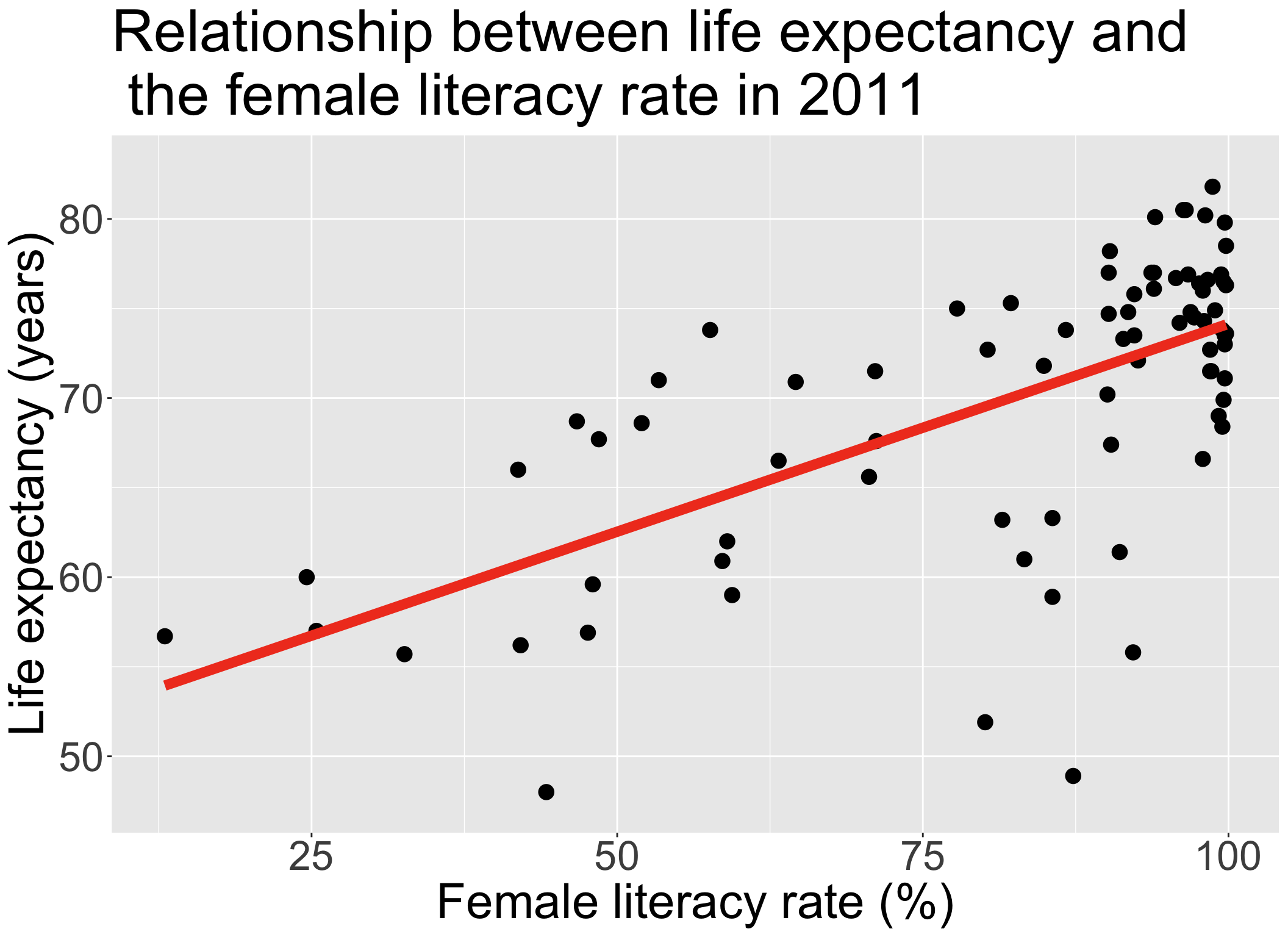
Let’s remind ourselves of the model that we have been working with

We have been looking at the association between life expectancy and female literacy rate
We used OLS to find the coefficient estimates of our best-fit line

\[Y = \beta_0 + \beta_1 X + \epsilon\]

term	estimate	std.error	statistic	p.value
(Intercept)	50.93	2.66	19.14	0.00
female_literacy_rate_2011	0.23	0.03	7.38	0.00

\[\begin{aligned} \widehat{Y} &= \widehat\beta_0 + \widehat\beta_1 \cdot X\\ \widehat{\text{life expectancy}} &= 50.9 + 0.232 \cdot \text{female literacy rate} \end{aligned}\]

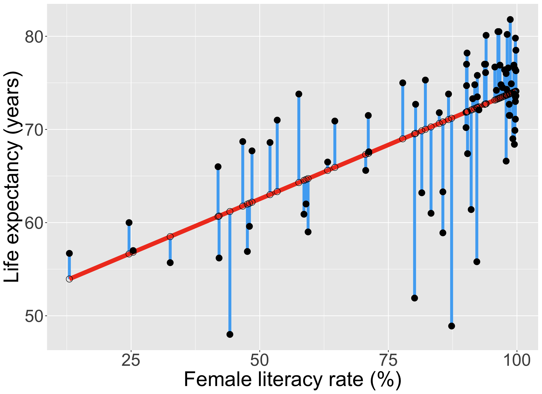
Our residuals will help us a lot in our diagnostics!

The residuals \(\widehat\epsilon_i\) are the vertical distances between
- the observed data \((X_i, Y_i)\)
- the fitted values (regression line) \(\widehat{Y}_i = \widehat\beta_0 + \widehat\beta_1 X_i\)

\[ \widehat\epsilon_i =Y_i - \widehat{Y}_i \text{, for } i=1, 2, ..., n \]

`augment()`: getting extra information on the fitted model

Run model1 through augment() (model1 is input)
- So we assigned model1 as the output of the lm() function (model1 is output)
Will give us values about each observation in the context of the fitted regression model
- cook’s distance (.cooksd), fitted value (.fitted, \(\widehat{Y}_i\)), leverage (.hat), residual (.resid), standardized residuals (.std.resid)

aug1 <- augment(model1) 
glimpse(aug1)

Rows: 80
Columns: 9
$ .rownames                  <chr> "1", "2", "5", "6", "7", "8", "14", "22", "…
$ life_expectancy_years_2011 <dbl> 56.7, 76.7, 60.9, 76.9, 76.0, 73.8, 71.0, 7…
$ female_literacy_rate_2011  <dbl> 13.0, 95.7, 58.6, 99.4, 97.9, 99.5, 53.4, 9…
$ .fitted                    <dbl> 53.94643, 73.14897, 64.53453, 74.00809, 73.…
$ .resid                     <dbl> 2.7535654, 3.5510294, -3.6345319, 2.8919074…
$ .hat                       <dbl> 0.13628996, 0.01768176, 0.02645854, 0.02077…
$ .sigma                     <dbl> 6.172684, 6.168414, 6.167643, 6.172935, 6.1…
$ .cooksd                    <dbl> 1.835891e-02, 3.062372e-03, 4.887448e-03, 2…
$ .std.resid                 <dbl> 0.48238134, 0.58332052, -0.59972251, 0.4757…

RDocumentation on the augment() function.

Revisiting our LINE assumptions

[L] Linearity of relationship between variables

Check if there is a linear relationship between the mean response (Y) and the explanatory variable (X)

[I] Independence of the \(Y\) values

Check that the observations are independent

[N] Normality of the \(Y\)’s given \(X\) (residuals)

Check that the responses (at each level X) are normally distributed

Usually measured through the residuals

[E] Equality of variance of the residuals (homoscedasticity)

Check that the variance (or standard deviation) of the responses is equal for all levels of X

Usually measured through the residuals

Learning Objectives

Use visualizations and cut off points to flag potentially influential points using residuals, leverage, and Cook’s distance

Handle influential points and assumption violations by checking data errors, reassessing the model, and making data transformations.
Implement a model with data transformations and determine if it improves the model fit.

Influential points

Outliers

An observation (\(X_i, Y_i\)) whose response \(Y_i\) does not follow the general trend of the rest of the data

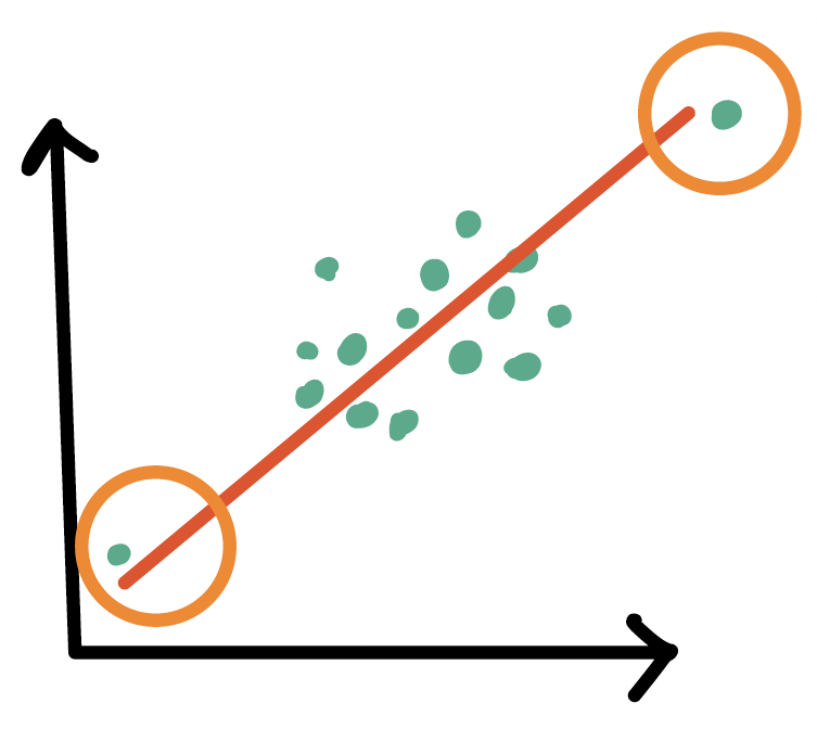
High leverage observations

An observation (\(X_i, Y_i\)) whose predictor \(X_i\) has an extreme value
\(X_i\) can be an extremely high or low value compared to the rest of the observations

Outliers

An observation (\(X_i, Y_i\)) whose response \(Y_i\) does not follow the general trend of the rest of the data
How do we determine if a point is an outlier?
- Scatterplot of \(Y\) vs. \(X\)
- Followed by evaluation of its residual (and standardized residual)

Use the internally standardized residual (aka studentized residual) to determine if an observation is an outlier

Poll Everywhere Question 1

Identifying outliers

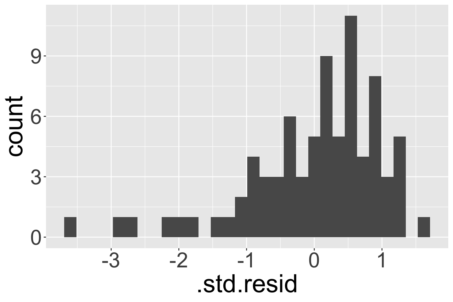
Internally standardized residual

\[ r_i = \frac{\widehat\epsilon_i}{\sqrt{\widehat\sigma^2(1-h_{ii})}} \]

We flag an observation if the standardized residual is “large”
- Different sources will define “large” differently
- PennState site uses \(|r_i| > 3\)
- autoplot() shows the 3 observations with the highest standardized residuals
- Other sources use \(|r_i| > 2\), which is a little more conservative

ggplot(data = aug1) + 
  geom_histogram(aes(x = .std.resid))

Countries that are outliers (\(|r_i| > 2\))

We can identify the countries that are outliers

aug1 %>% 
  filter(abs(.std.resid) > 2)

# A tibble: 4 × 10
  .rownames country     life_expectancy_year…¹ female_literacy_rate…² .std.resid
  <chr>     <chr>                        <dbl>                  <dbl>      <dbl>
1 33        Central Af…                   48                     44.2      -2.20
2 152       South Afri…                   55.8                   92.2      -2.71
3 161       Swaziland                     48.9                   87.3      -3.65
4 187       Zimbabwe                      51.9                   80.1      -2.89
# ℹ abbreviated names: ¹life_expectancy_years_2011, ²female_literacy_rate_2011
# ℹ 5 more variables: .fitted <dbl>, .resid <dbl>, .hat <dbl>, .sigma <dbl>,
#   .cooksd <dbl>

High leverage observations

An observation (\(X_i, Y_i\)) whose response \(X_i\) is considered “extreme” compared to the other values of \(X\)

How do we determine if a point has high leverage?
- Scatterplot of \(Y\) vs. \(X\)
- Calculating the leverage of each observation

Leverage \(h_i\)

Values of leverage are: \(0 \leq h_i \leq 1\)
We flag an observation if the leverage is “high”
- Different sources will define “high” differently
- Some textbooks use \(h_i > 4/n\) where \(n\) = sample size
- Some people suggest \(h_i > 6/n\)
- PennState site uses \(h_i > 3p/n\) where \(p\) = number of regression coefficients

aug1 = aug1 %>% relocate(.hat, .after = female_literacy_rate_2011)
aug1 %>% arrange(desc(.hat))

# A tibble: 80 × 10
   .rownames country        life_expectancy_year…¹ female_literacy_rate…²   .hat
   <chr>     <chr>                           <dbl>                  <dbl>  <dbl>
 1 1         Afghanistan                      56.7                   13   0.136 
 2 104       Mali                             60                     24.6 0.0980
 3 34        Chad                             57                     25.4 0.0956
 4 146       Sierra Leone                     55.7                   32.6 0.0757
 5 62        Gambia                           66                     41.9 0.0540
 6 70        Guinea-Bissau                    56.2                   42.1 0.0536
 7 33        Central Afric…                   48                     44.2 0.0493
 8 118       Nepal                            68.7                   46.7 0.0446
 9 42        Cote d'Ivoire                    56.9                   47.6 0.0430
10 169       Togo                             59.6                   48   0.0422
# ℹ 70 more rows
# ℹ abbreviated names: ¹life_expectancy_years_2011, ²female_literacy_rate_2011
# ℹ 5 more variables: .std.resid <dbl>, .fitted <dbl>, .resid <dbl>,
#   .sigma <dbl>, .cooksd <dbl>

Countries with high leverage (\(h_i > 4/n\))

We can look at the countries that have high leverage

aug1 %>% 
  filter(.hat > 4/80) %>%
  arrange(desc(.hat))

# A tibble: 6 × 10
  .rownames country       life_expectancy_years_…¹ female_literacy_rate…²   .hat
  <chr>     <chr>                            <dbl>                  <dbl>  <dbl>
1 1         Afghanistan                       56.7                   13   0.136 
2 104       Mali                              60                     24.6 0.0980
3 34        Chad                              57                     25.4 0.0956
4 146       Sierra Leone                      55.7                   32.6 0.0757
5 62        Gambia                            66                     41.9 0.0540
6 70        Guinea-Bissau                     56.2                   42.1 0.0536
# ℹ abbreviated names: ¹life_expectancy_years_2011, ²female_literacy_rate_2011
# ℹ 5 more variables: .std.resid <dbl>, .fitted <dbl>, .resid <dbl>,
#   .sigma <dbl>, .cooksd <dbl>

Poll Everywhere Question 2

Countries with high leverage (\(h_i > 4/n\))

Label only countries with large leverage:

ggplot(aug1, aes(x = female_literacy_rate_2011, y = life_expectancy_years_2011,
                 label = country)) +
  geom_point() +
  geom_smooth(method = "lm", color = "darkgreen") +
  geom_text(aes(label = ifelse(.hat > 0.05, as.character(country), ''))) +
  geom_vline(xintercept = mean(aug1$female_literacy_rate_2011), color = "grey") +
  geom_hline(yintercept = mean(aug1$life_expectancy_years_2011), color = "grey")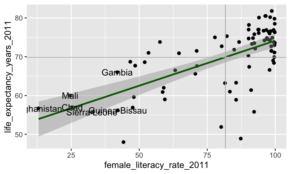

What does the model look like without the high leverage points?

Sensitivity analysis removing countries with high leverage

model1_lowlev <- lm(life_expectancy_years_2011 ~ female_literacy_rate_2011,
                    data = aug1_lowlev)
tidy(model1_lowlev) %>% gt() %>% # Without high-leverage points
 tab_options(table.font.size = 40) %>%
 fmt_number(decimals = 3)

term	estimate	std.error	statistic	p.value
(Intercept)	49.563	3.888	12.746	0.000
female_literacy_rate_2011	0.247	0.044	5.562	0.000

tidy(model1) %>% gt() %>% # With high leverage points
 tab_options(table.font.size = 40) %>%
 fmt_number(decimals = 3)

term	estimate	std.error	statistic	p.value
(Intercept)	50.928	2.660	19.143	0.000
female_literacy_rate_2011	0.232	0.031	7.377	0.000

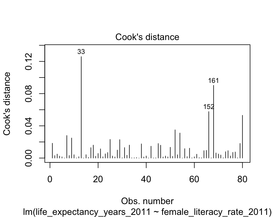
Cook’s distance

Measures the overall influence of an observation

Attempts to measure how much influence a single observation has over the fitted model
- Measures how all fitted values change when the \(ith\) observation is removed from the model
- Combines leverage and outlier information

Identifying points with high Cook’s distance

The Cook’s distance for the \(i^{th}\) observation is

\[d_i = \frac{h_i}{2(1-h_i)} \cdot r_i^2\] where \(h_i\) is the leverage and \(r_i\) is the studentized residual

Another rule for Cook’s distance that is not strict:
- Investigate observations that have \(d_i > 1\)
Cook’s distance values are already in the augment tibble: .cooksd

aug1 = aug1 %>% relocate(.cooksd, .after = female_literacy_rate_2011)
aug1 %>% arrange(desc(.cooksd))

# A tibble: 80 × 10
   .rownames country       life_expectancy_year…¹ female_literacy_rate…² .cooksd
   <chr>     <chr>                          <dbl>                  <dbl>   <dbl>
 1 33        Central Afri…                   48                     44.2  0.126 
 2 161       Swaziland                       48.9                   87.3  0.0903
 3 152       South Africa                    55.8                   92.2  0.0577
 4 187       Zimbabwe                        51.9                   80.1  0.0531
 5 114       Morocco                         73.8                   57.6  0.0350
 6 118       Nepal                           68.7                   46.7  0.0311
 7 14        Bangladesh                      71                     53.4  0.0280
 8 23        Botswana                        58.9                   85.6  0.0249
 9 54        Equatorial G…                   61.4                   91.1  0.0231
10 62        Gambia                          66                     41.9  0.0228
# ℹ 70 more rows
# ℹ abbreviated names: ¹life_expectancy_years_2011, ²female_literacy_rate_2011
# ℹ 5 more variables: .hat <dbl>, .std.resid <dbl>, .fitted <dbl>,
#   .resid <dbl>, .sigma <dbl>

Plotting Cook’s Distance

# plot(model) shows figures similar to autoplot()
# adds on Cook's distance though
plot(model1, which = 4)

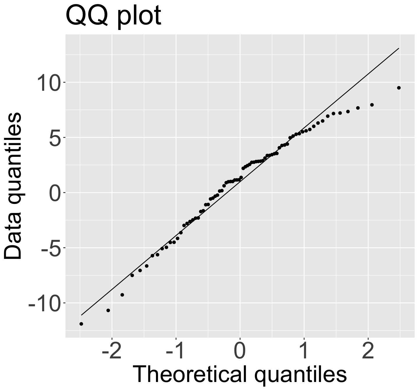
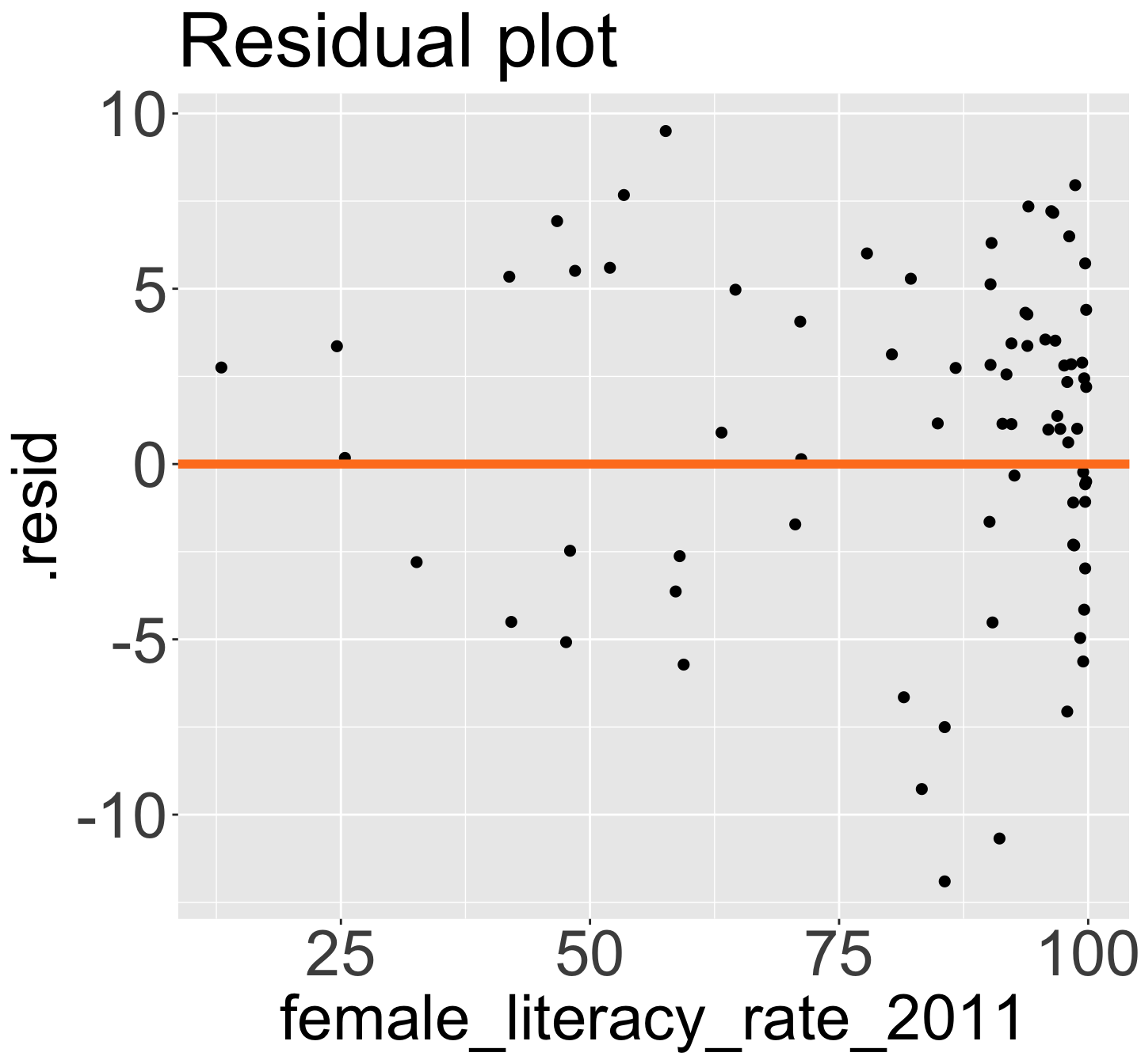
Model without those 4 points: QQ Plot, Residual plot

model1_lowcd <- lm(life_expectancy_years_2011 ~ female_literacy_rate_2011,
                    data = aug1_lowcd)
tidy(model1_lowcd) %>% gt() %>% # Without high-leverage points
 tab_options(table.font.size = 40) %>%
 fmt_number(decimals = 3)

term	estimate	std.error	statistic	p.value
(Intercept)	52.388	2.078	25.208	0.000
female_literacy_rate_2011	0.226	0.024	9.208	0.000

tidy(model1) %>% gt() %>% # With high leverage points
 tab_options(table.font.size = 40) %>%
 fmt_number(decimals = 3)

term	estimate	std.error	statistic	p.value
(Intercept)	50.928	2.660	19.143	0.000
female_literacy_rate_2011	0.232	0.031	7.377	0.000

Model without those 4 points: QQ Plot, Residual plot

I am okay with this!

And don’t forget: we may want more variables in our model!
You do not need to produce plots with the influential points taken out

Summary of how we identify influential points

Use scatterplot of \(Y\) vs. \(X\) to see if any points fall outside of range we expect
Use standardized residuals, leverage, and Cook’s distance to further identify those points
Look at the models run with and without the identified points to check for drastic changes
- Look at QQ plot and residuals to see if assumptions hold without those points
- Look at coefficient estimates to see if they change in sign and large magnitude

Next: how to handle? It’s a little wishy washy

Learning Objectives

Use visualizations and cut off points to flag potentially influential points using residuals, leverage, and Cook’s distance

Handle influential points and assumption violations by checking data errors, reassessing the model, and making data transformations.

Implement a model with data transformations and determine if it improves the model fit.

How do we deal with influential points?

It’s always weird to be using numbers to help you diagnose an issue, but the issue kinda gets unresolved
If an observation is influential, we can check data errors:
- Was there a data entry or collection problem?
- If you have reason to believe that the observation does not hold within the population (or gives you cause to redefine your population)
If an observation is influential, we can check our model:
- Did you leave out any important predictors?
- Should you consider adding some interaction terms?
- Is there any nonlinearity that needs to be modeled?
Basically, deleting an observation should be justified outside of the numbers!
- If it’s an honest data point, then it’s giving us important information!
A really well thought out explanation from StackExchange

When we have detected problems in our model…

We have talked about influential points
We have talked about identifying issues with our LINE assumptions

What are our options once we have identified issues in our linear regression model?

See if we need to add predictors to our model
- Nicky’s thought for our life expectancy example
Try a transformation if there is an issue with linearity or normality
Try a transformation if there is unequal variance
Try a weighted least squares approach if unequal variance (might be lesson at end of course)
Try a robust estimation procedure if we have a lot of outlier issues (outside scope of class)

Learning Objectives

Use visualizations and cut off points to flag potentially influential points using residuals, leverage, and Cook’s distance
Handle influential points and assumption violations by checking data errors, reassessing the model, and making data transformations.

Implement a model with data transformations and determine if it improves the model fit.

Transformations

When we have issues with our LINE (mostly linearity, normality, or equality of variance) assumptions
- We can use transformations to improve the fit of the model
Transformations can…
- Make the relationship more linear
- Make the residuals more normal
- “Stabilize” the variance so that it is more constant
- It can also bring in or reduce outliers
We can transform the dependent (\(Y\)) variable of the independent (\(X\)) variable
- Usually we want to try transforming the \(X\) first

Requires trial and error!!
Major drawback: interpreting the model becomes harder!

Common transformations

Tukey’s transformation (power) ladder
- Use R’s gladder() command from the describedata package

Power p	-3	-2	-1	-1/2	0	1/2	1	2	3
	\(\frac{1}{x^3}\)	\(\frac{1}{x^2}\)	\(\frac{1}{x}\)	\(\frac{1}{\sqrt{x}}\)	\(\log(x)\)	\(\sqrt{x}\)	\(x\)	\(x^2\)	\(x^3\)

How to use the power ladder for the general distribution shape
- If data are skewed left, we need to compress smaller values towards the rest of the data
  - Go “up” ladder to transformations with power > 1
- If data are skewed right, we need to compress larger values towards the rest of the data
  - Go “down” ladder to transformations with power < 1

How to use the power ladder for heteroscedasticity
- If higher \(X\) values have more spread
  - Compress larger values towards the rest of the data
  - Go “down” ladder to transformations with power < 1
- If lower \(X\) values have more spread
  - Compress smaller values towards the rest of the data
  - Go “up” ladder to transformations with power > 1

Poll Everywhere Question 3

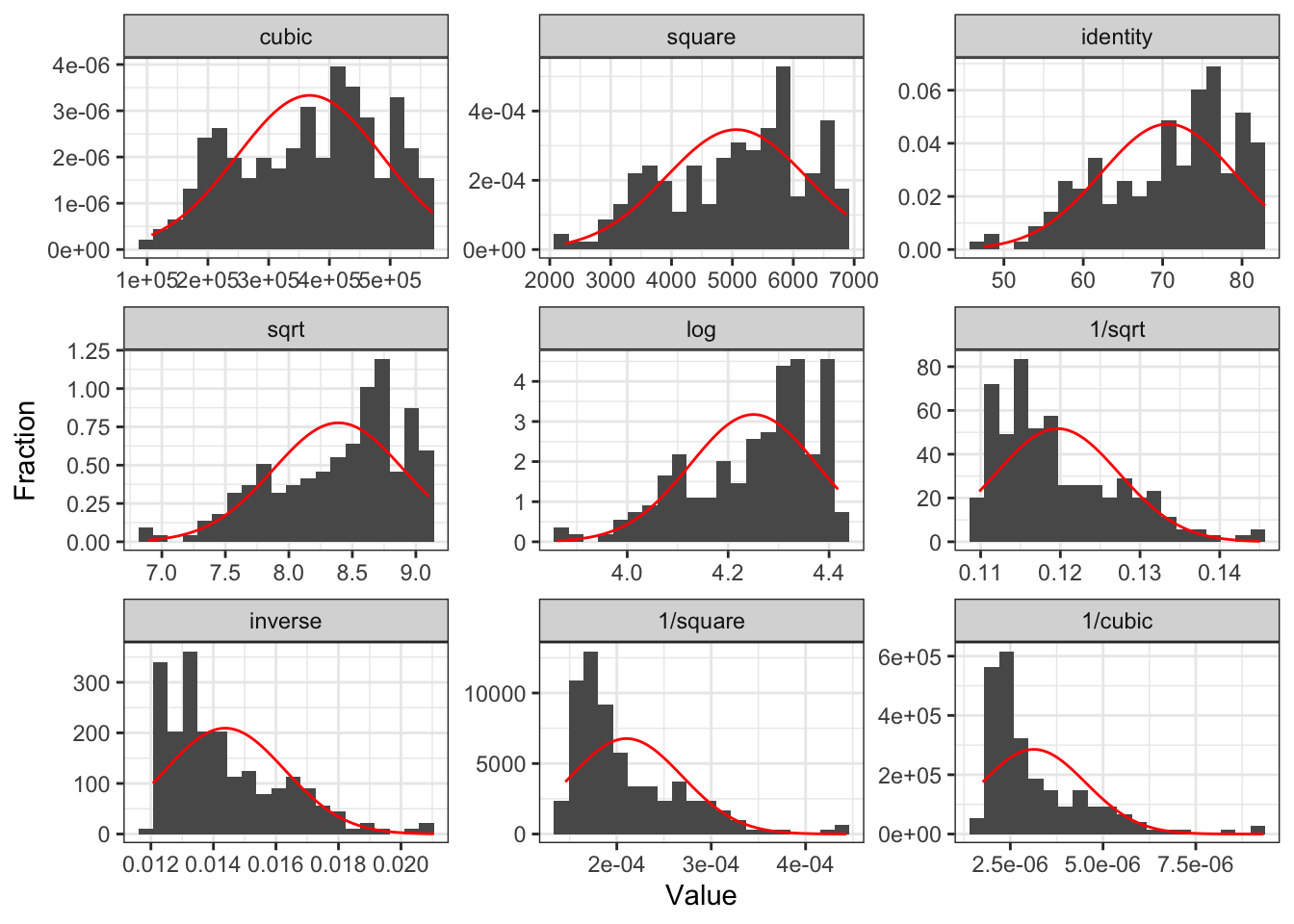
Transform dependent variable?

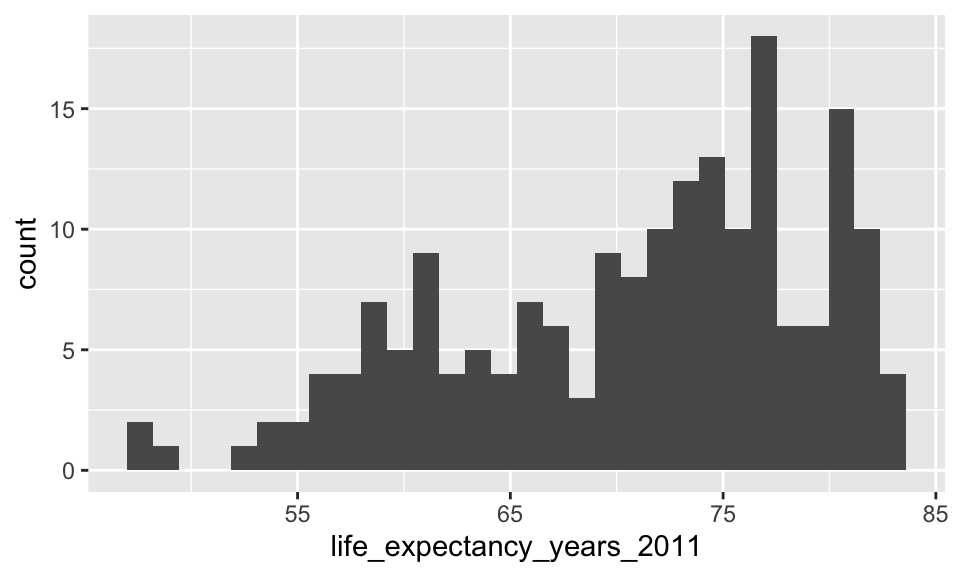
ggplot(gapm, aes(x = life_expectancy_years_2011)) +
  geom_histogram()

`gladder()` of life expectancy

gladder(gapm$life_expectancy_years_2011)

Transform independent variable?

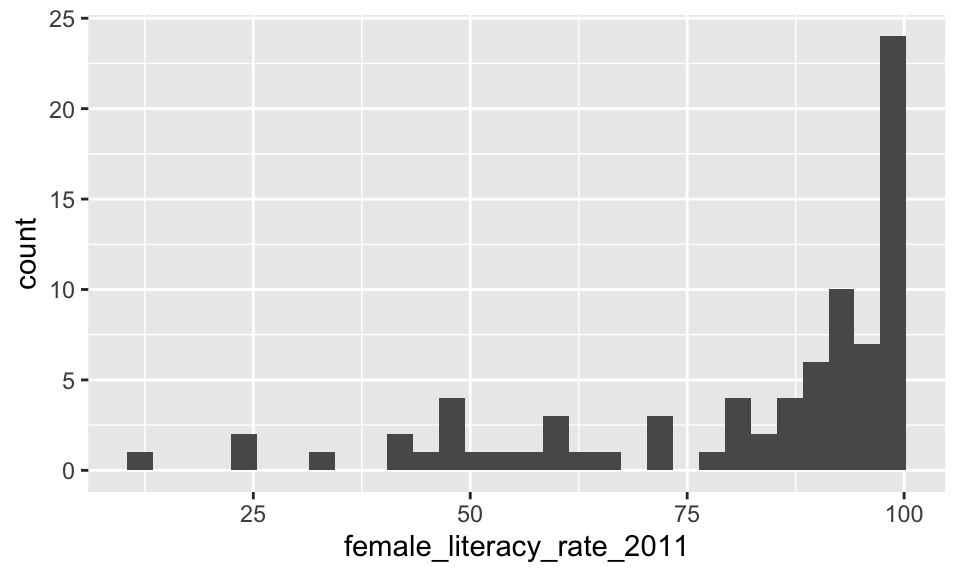
ggplot(gapm, aes(x = female_literacy_rate_2011)) +
  geom_histogram()

`gladder()` of female literacy rate

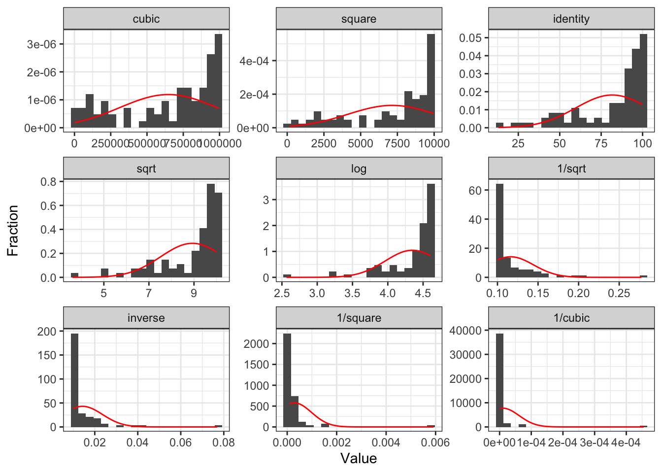
gladder(gapm$female_literacy_rate_2011)

Tips

Recall, assessing our LINE assumptions are not on \(Y\) alone!!
- We can use gladder() to get a sense of what our transformations will do to the data, but we need to check with our residuals again!!
Transformations usually work better if all values are positive (or negative)
If observation has a 0, then we cannot perform certain transformations
Log function only defined for positive values
- We might take the \(log(X+1)\) if \(X\) includes a 0 value
When we make cubic or sqaure transformations, we MUST include the original \(X\)
- We do not do this for \(Y\) though

Add quadratic and cubic transformations to dataset

Helpful to make a new variable with the transformation in your dataset

gapm <- gapm %>% 
  mutate(LE_2 = life_expectancy_years_2011^2,
         LE_3 = life_expectancy_years_2011^3,
         FLR_2 = female_literacy_rate_2011^2,
         FLR_3 = female_literacy_rate_2011^3)

glimpse(gapm)

Rows: 188
Columns: 8
$ country                    <chr> "Afghanistan", "Albania", "Algeria", "Andor…
$ life_expectancy_years_2011 <dbl> 56.7, 76.7, 76.7, 82.6, 60.9, 76.9, 76.0, 7…
$ female_literacy_rate_2011  <dbl> 13.0, 95.7, NA, NA, 58.6, 99.4, 97.9, 99.5,…
$ .rownames                  <chr> "1", "2", "3", "4", "5", "6", "7", "8", "9"…
$ LE_2                       <dbl> 3214.89, 5882.89, 5882.89, 6822.76, 3708.81…
$ LE_3                       <dbl> 182284.3, 451217.7, 451217.7, 563560.0, 225…
$ FLR_2                      <dbl> 169.00, 9158.49, NA, NA, 3433.96, 9880.36, …
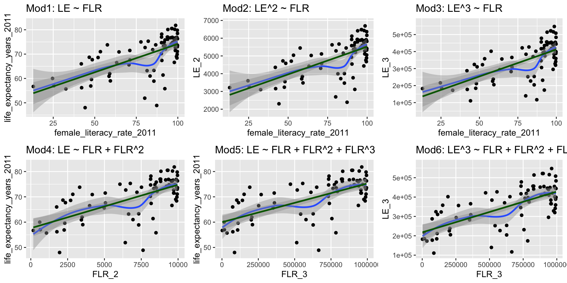
$ FLR_3                      <dbl> 2197.0, 876467.5, NA, NA, 201230.1, 982107.…

We are going to compare a few different models with transformations

We are going to call life expectancy \(LE\) and female literacy rate \(FLR\)

Model 1: \(LE = \beta_0 + \beta_1 FLR + \epsilon\)
Model 2: \(LE^2 = \beta_0 + \beta_1 FLR + \epsilon\)
Model 3: \(LE^3 = \beta_0 + \beta_1 FLR + \epsilon\)
Model 4: \(LE = \beta_0 + \beta_1 FLR + \beta_2 FLR^2 +\epsilon\)
Model 5: \(LE = \beta_0 + \beta_1 FLR + \beta_2 FLR^2 +\beta_3 FLR^3 +\epsilon\)
Model 6: \(LE^3 = \beta_0 + \beta_1 FLR + \beta_2 FLR^2 +\beta_3 FLR^3 +\epsilon\)

Poll Everywhere Question 4

Compare Scatterplots: does linearity improve?

Run models with transformations: examples

Model 2: \(LE^2 = \beta_0 + \beta_1 FLR + \epsilon\)

model2 <- lm(LE_2 ~ female_literacy_rate_2011,
             data = gapm)

term	estimate	std.error	statistic	p.value
(Intercept)	2,401.272	352.070	6.820	0.000
female_literacy_rate_2011	31.174	4.166	7.484	0.000

Model 6: \(LE^3 = \beta_0 + \beta_1 FLR + \beta_2 FLR^2 +\beta_3 FLR^3 +\epsilon\)

model6 <- lm(LE_3 ~ 
               female_literacy_rate_2011 + FLR_2 + FLR_3,
             data = gapm)

term	estimate	std.error	statistic	p.value
(Intercept)	67,691.796	149,056.945	0.454	0.651
female_literacy_rate_2011	8,092.133	8,473.154	0.955	0.343
FLR_2	−128.596	147.876	−0.870	0.387
FLR_3	0.840	0.794	1.059	0.293

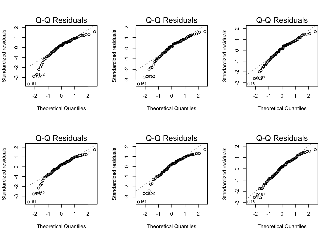
Normal Q-Q plots comparison

Residual plots comparison

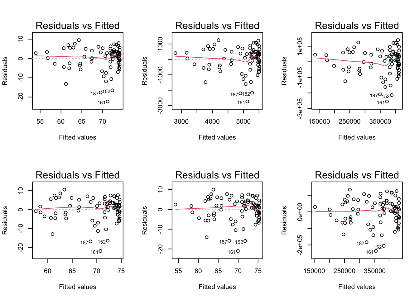
Summary of transformations

If the model without the transformation is blatantly violating a LINE assumption
- Then a transformation is a good idea
If the model without a transformation is not following the LINE assumptions very well, but is mostly okay
- Then try to avoid a transformation
- Think about what predictors might need to be added
- Especially if you keep seeing the same points as influential
If interpretability is important in your final work, then transformations are not a great solution

Reference: all run models

Model 2: \(LE^2 = \beta_0 + \beta_1 FLR + \epsilon\)

model2 <- lm(LE_2 ~ female_literacy_rate_2011,
             data = gapm)

tidy(model2) %>% gt()

term	estimate	std.error	statistic	p.value
(Intercept)	2401.27207	352.069818	6.820443	1.726640e-09
female_literacy_rate_2011	31.17351	4.165624	7.483514	9.352191e-11

Model 3: \(LE^3 \sim FLR\)

model3 <- lm(LE_3 ~ female_literacy_rate_2011,
             data = gapm)

tidy(model3) %>% gt()

term	estimate	std.error	statistic	p.value
(Intercept)	95453.189	35631.6898	2.678885	9.005716e-03
female_literacy_rate_2011	3166.481	421.5875	7.510853	8.285324e-11

Model 4: \(LE \sim FLR + FLR^2\)

model4 <- lm(life_expectancy_years_2011 ~ 
               female_literacy_rate_2011 + FLR_2,
             data = gapm)

tidy(model4) %>% gt()

term	estimate	std.error	statistic	p.value
(Intercept)	57.030875456	6.282845592	9.07723652	8.512585e-14
female_literacy_rate_2011	0.019348795	0.201021963	0.09625215	9.235704e-01
FLR_2	0.001578649	0.001472592	1.07202008	2.870595e-01

Model 5: \(LE \sim FLR + FLR^2 + FLR^3\)

model5 <- lm(life_expectancy_years_2011 ~ 
               female_literacy_rate_2011 + FLR_2 + FLR_3,
             data = gapm)

tidy(model5) %>% gt()

term	estimate	std.error	statistic	p.value
(Intercept)	4.732796e+01	1.117939e+01	4.2335001	6.373341e-05
female_literacy_rate_2011	6.517986e-01	6.354934e-01	1.0256576	3.083065e-01
FLR_2	-9.952763e-03	1.109080e-02	-0.8973895	3.723451e-01
FLR_3	6.245016e-05	5.953283e-05	1.0490038	2.975008e-01

Model 6: \(LE^3 \sim FLR + FLR^2 + FLR^3\)

model6 <- lm(LE_3 ~ 
               female_literacy_rate_2011 + FLR_2 + FLR_3,
             data = gapm)

tidy(model6) %>% gt()

term	estimate	std.error	statistic	p.value
(Intercept)	67691.7963283	1.490569e+05	0.4541338	0.6510268
female_literacy_rate_2011	8092.1325988	8.473154e+03	0.9550320	0.3425895
FLR_2	-128.5960879	1.478757e+02	-0.8696230	0.3872447
FLR_3	0.8404736	7.937625e-01	1.0588477	0.2930229

SLR: Model Evaluation and Diagnostics

Learning Objectives

Let’s remind ourselves of the model that we have been working with

Our residuals will help us a lot in our diagnostics!

augment(): getting extra information on the fitted model

Revisiting our LINE assumptions

Learning Objectives

Influential points

Outliers

Poll Everywhere Question 1

Identifying outliers

Countries that are outliers (\(|r_i| > 2\))

High leverage observations

Leverage \(h_i\)

Countries with high leverage (\(h_i > 4/n\))

Poll Everywhere Question 2

Countries with high leverage (\(h_i > 4/n\))

What does the model look like without the high leverage points?

Cook’s distance

Identifying points with high Cook’s distance

Plotting Cook’s Distance

Model without those 4 points: QQ Plot, Residual plot

Model without those 4 points: QQ Plot, Residual plot

Summary of how we identify influential points

Learning Objectives

How do we deal with influential points?

When we have detected problems in our model…

Learning Objectives

Transformations

Common transformations

Poll Everywhere Question 3

Transform dependent variable?

gladder() of life expectancy

Transform independent variable?

gladder() of female literacy rate

Tips

Add quadratic and cubic transformations to dataset

We are going to compare a few different models with transformations

Poll Everywhere Question 4

Compare Scatterplots: does linearity improve?

Run models with transformations: examples

Normal Q-Q plots comparison

Residual plots comparison

Summary of transformations

Reference: all run models

`augment()`: getting extra information on the fitted model

`gladder()` of life expectancy

`gladder()` of female literacy rate