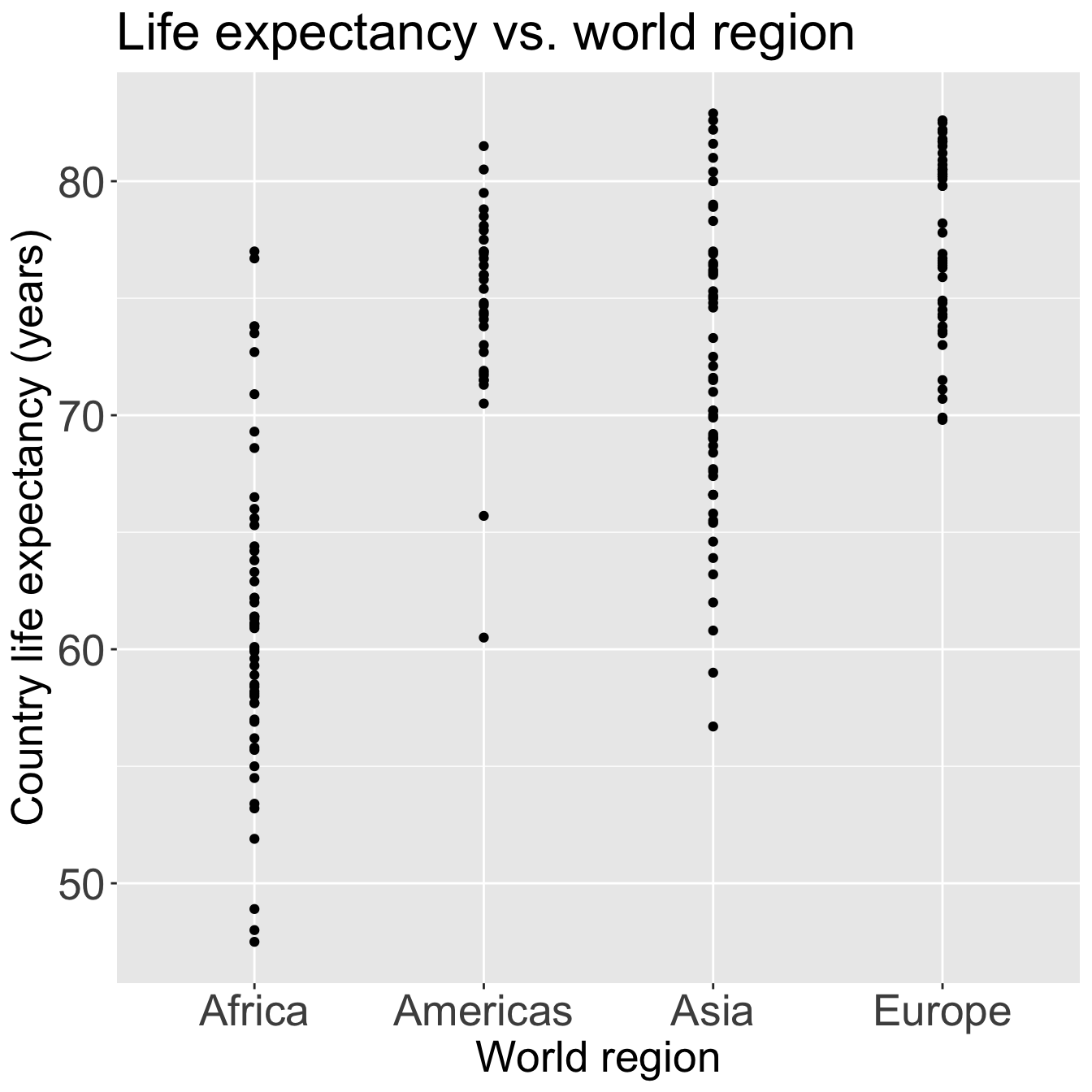
ggplot(gapm2, aes(x = four_regions, y = LifeExpectancyYrs)) +geom_point() +labs(x ="World region", y ="Country life expectancy (years)",title ="Life expectancy vs. world region") +theme(axis.title =element_text(size =20), axis.text =element_text(size =20), title =element_text(size =20))
Good option for visualization:
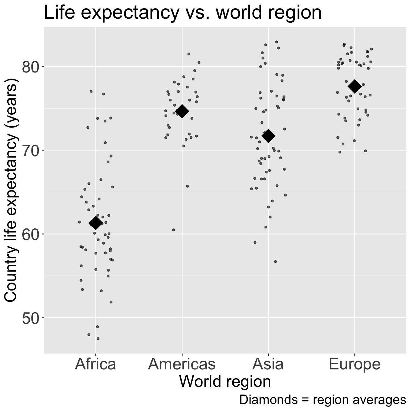
Code
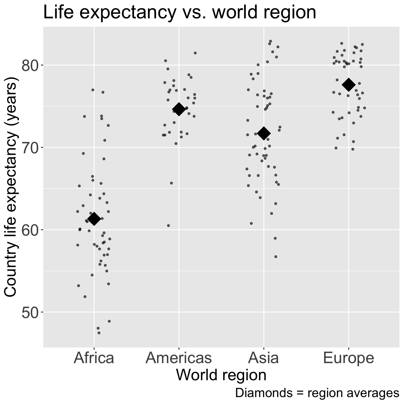
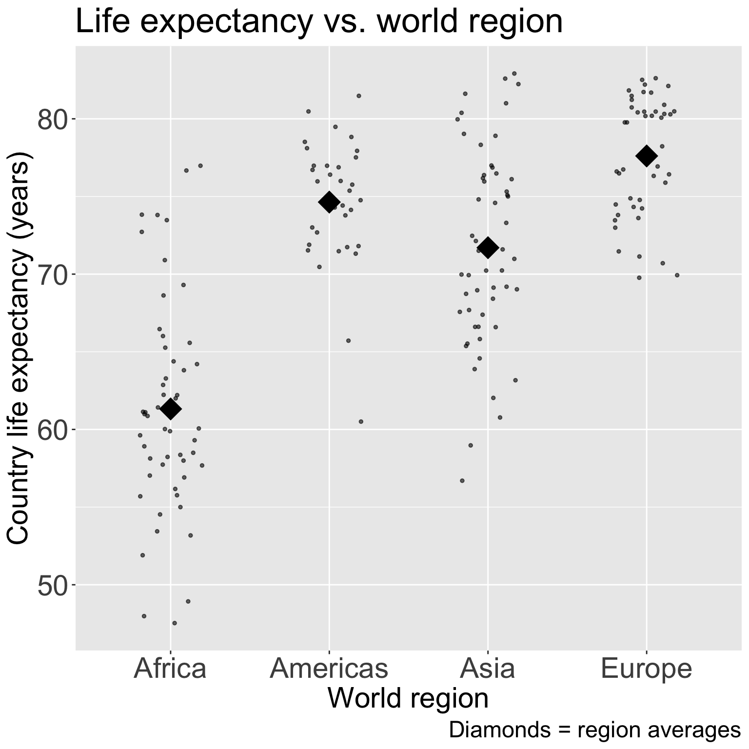
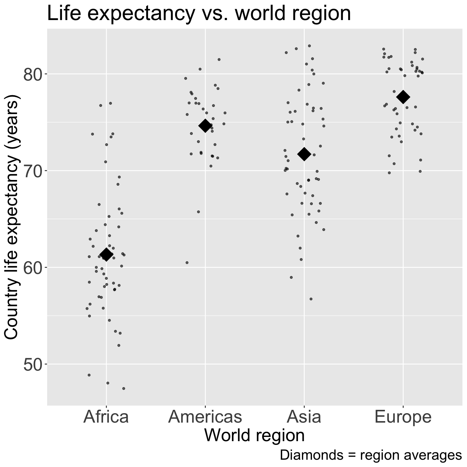
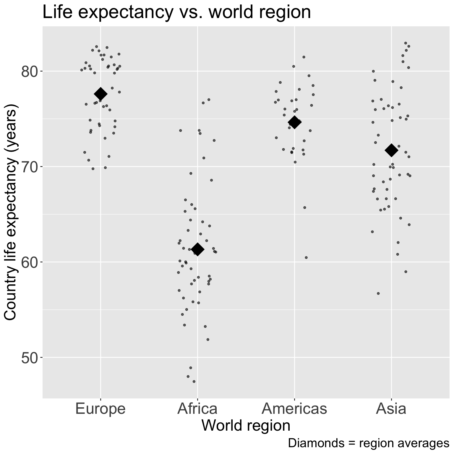
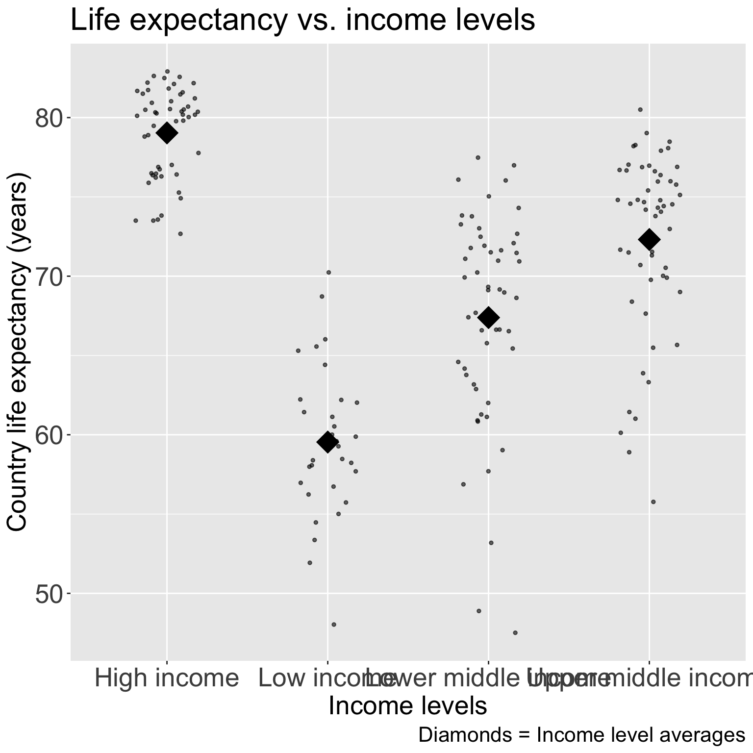
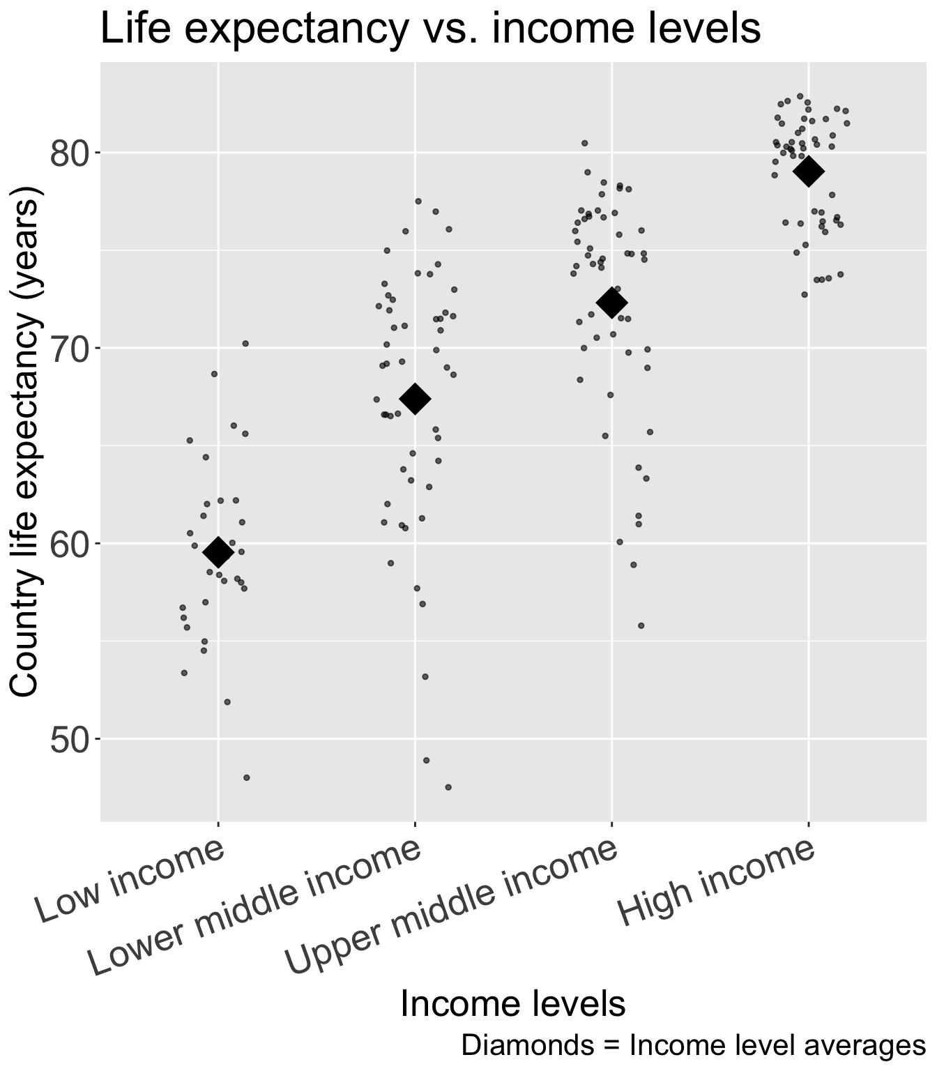
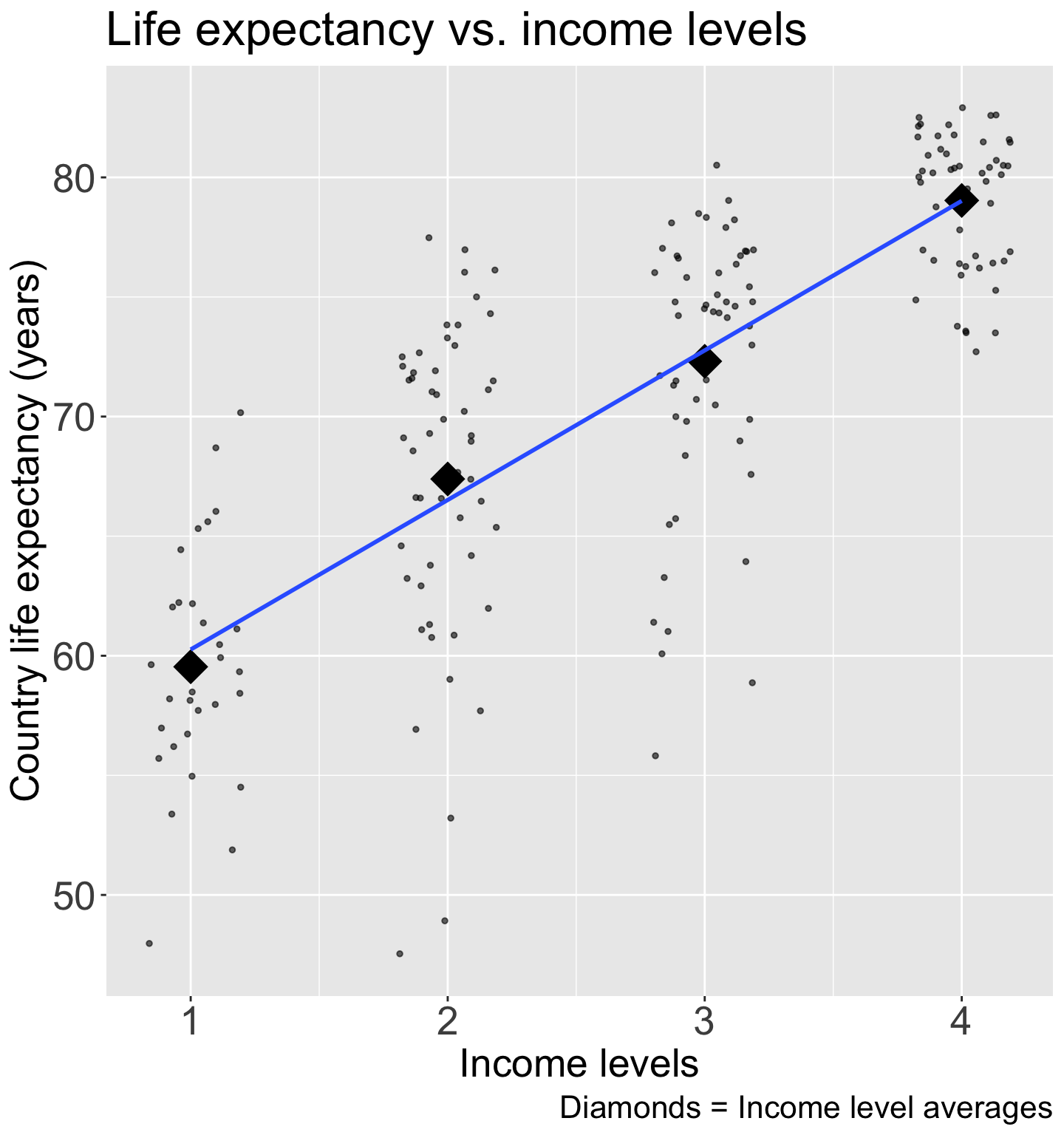
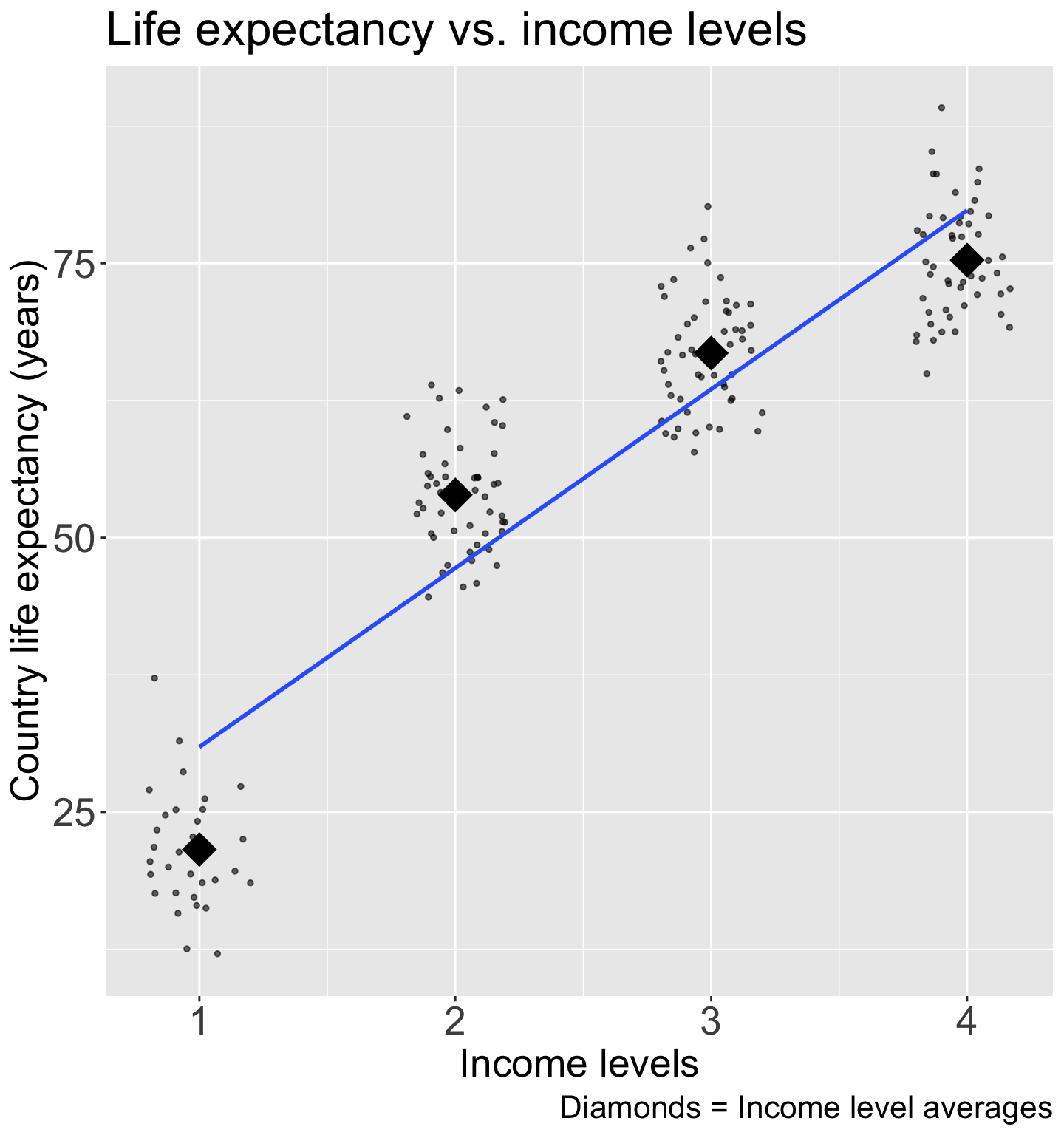
ggplot(gapm2, aes(x = four_regions, y = LifeExpectancyYrs)) +geom_jitter(size =1, alpha = .6, width =0.2) +stat_summary(fun = mean, geom ="point", size =8, shape =18) +labs(x ="World region", y ="Country life expectancy (years)",title ="Life expectancy vs. world region",caption ="Diamonds = region averages") +theme(axis.title =element_text(size =20), axis.text =element_text(size =20), title =element_text(size =20))
Good option for visualization:
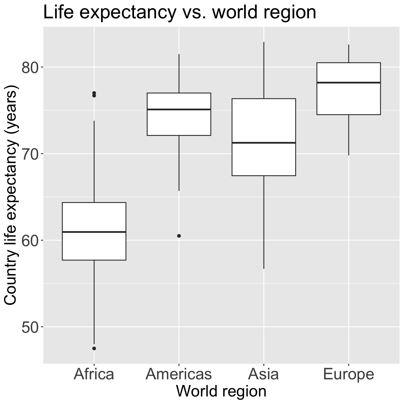
Code
ggplot(gapm2, aes(x = four_regions, y = LifeExpectancyYrs)) +geom_boxplot() +labs(x ="World region", y ="Country life expectancy (years)",title ="Life expectancy vs. world region") +theme(axis.title =element_text(size =20), axis.text =element_text(size =20), title =element_text(size =20))
Linear regression with a categorical covariate
When using a categorical covariate/predictor (that is not ordered),
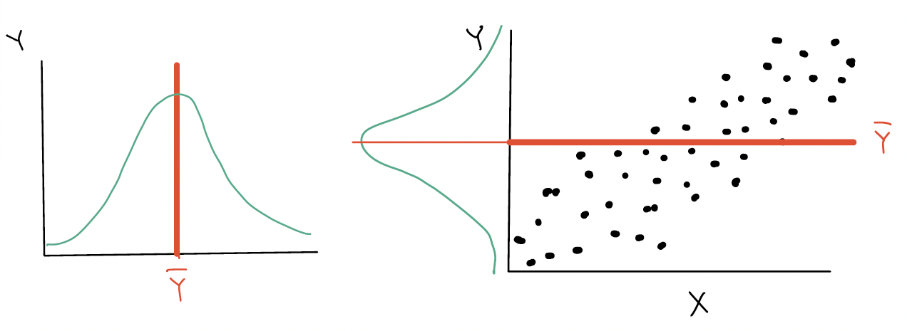
We do NOT, technically, find a best-fit line
Instead we model the means of the outcome
For the different levels of the categorical variable
In 511, we used Kruskal-Wallis test and our ANOVA table to test if groups means were statistically different from one another
We can do this using linear models AND we can include other variable in the model
There are different ways to code categorical variables
Reference cell coding (sometimes called dummy coding)
Compares each level of a variable to the omitted (reference) level
Effect coding (sometimes called sum coding or deviation coding)
Compares deviations from the grand mean
Ordinal encoding (sometimes called scoring)
Categories have a natural, even spaced ordering
If you want to learn more about these and other coding schemes:
# means of each level of `four_regions`gapm2_ave <- gapm2 %>%group_by(four_regions) %>%summarise(life_ave =mean(LifeExpectancyYrs))# mean of `africa`mean_africa <- gapm2_ave %>%filter(four_regions =="Africa") %>%pull(life_ave)# differences in means between levels of `four_regions` and `africa`gapm2_ave_diff <- gapm2_ave %>%mutate(`Difference with Africa`= life_ave - mean_africa) %>%rename(`World regions`= four_regions, `Average life expectancy`= life_ave)# At the beginning of the Rmd we loaded knitr, which is where the kable command is from# library(knitr)gapm2_ave_diff %>%kable(digits =1,format ="markdown" )
Observed values\(y\) are the values in the dataset
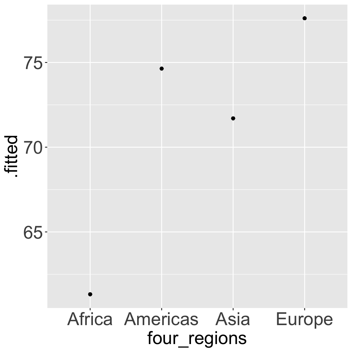
Fitted values\(\widehat{y}\) are the values that fall on the best-fit line for a specific value of x are the means of the outcome stratified by the categorical predictor’s levels
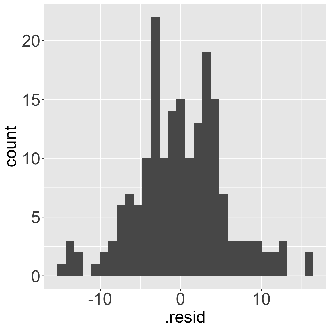
Residuals\(y - \widehat{y}\) are the differences between the two