Lesson 11: Interactions
2024-02-14
Let’s map that to our regression analysis process

![]()
![]()
Model Selection
Building a model
Selecting variables
Prediction vs interpretation
Comparing potential models
Model Fitting
Find best fit line
Using OLS in this class
Parameter estimation
Categorical covariates
Interactions
Model Evaluation
- Evaluation of model fit
- Testing model assumptions
- Residuals
- Transformations
- Influential points
- Multicollinearity
Model Use (Inference)
- Inference for coefficients
- Hypothesis testing for coefficients
- Inference for expected \(Y\) given \(X\)
Recall our data and the main relationship
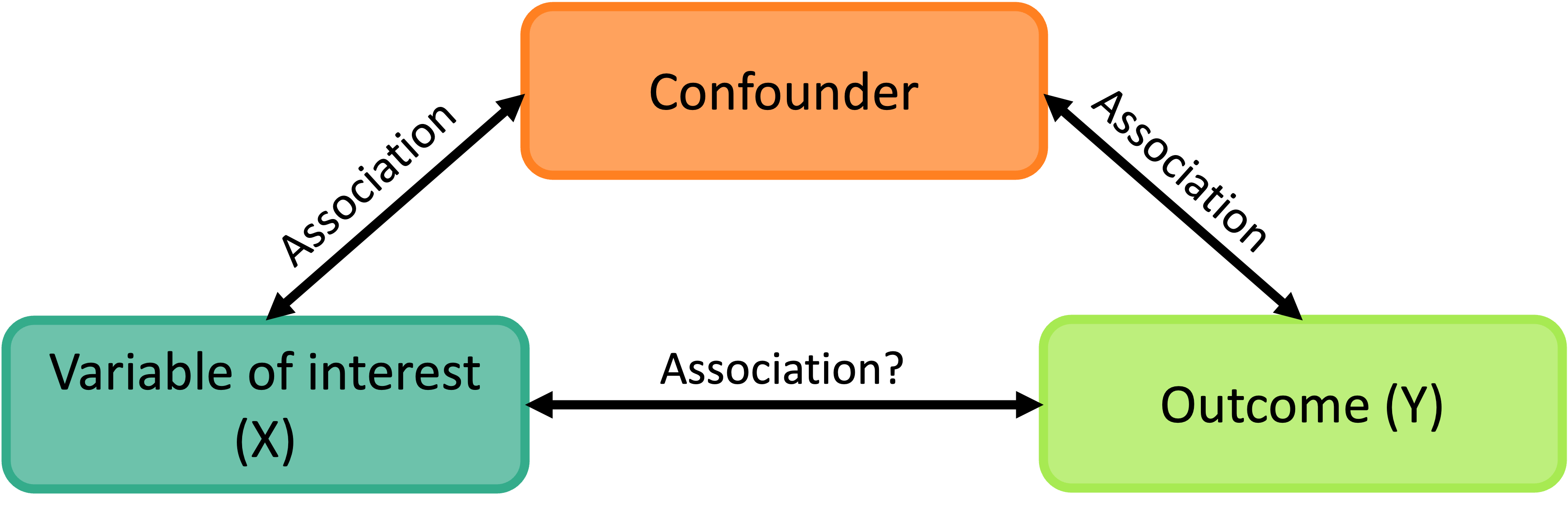
What is a confounder?
A confounding variable, or confounder, is a factor/variable that wholly or partially accounts for the observed effect of the risk factor on the outcome
A confounder must be…
- Related to the outcome Y, but not a consequence of Y
- Related to the explanatory variable X, but not a consequence of X
What is an effect modifier?
An additional variable in the model
- Outside of the main relationship between \(Y\) and \(X_1\) that we are studying
An effect modifier will change the effect of \(X_1\) on \(Y\) depending on its value
Aka: as the effect modifier’s values change, so does the association between \(Y\) and \(X_1\)
So the coefficient estimating the relationship between \(Y\) and \(X_1\) changes with another variable
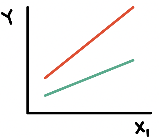
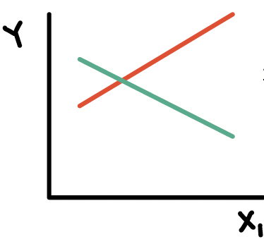
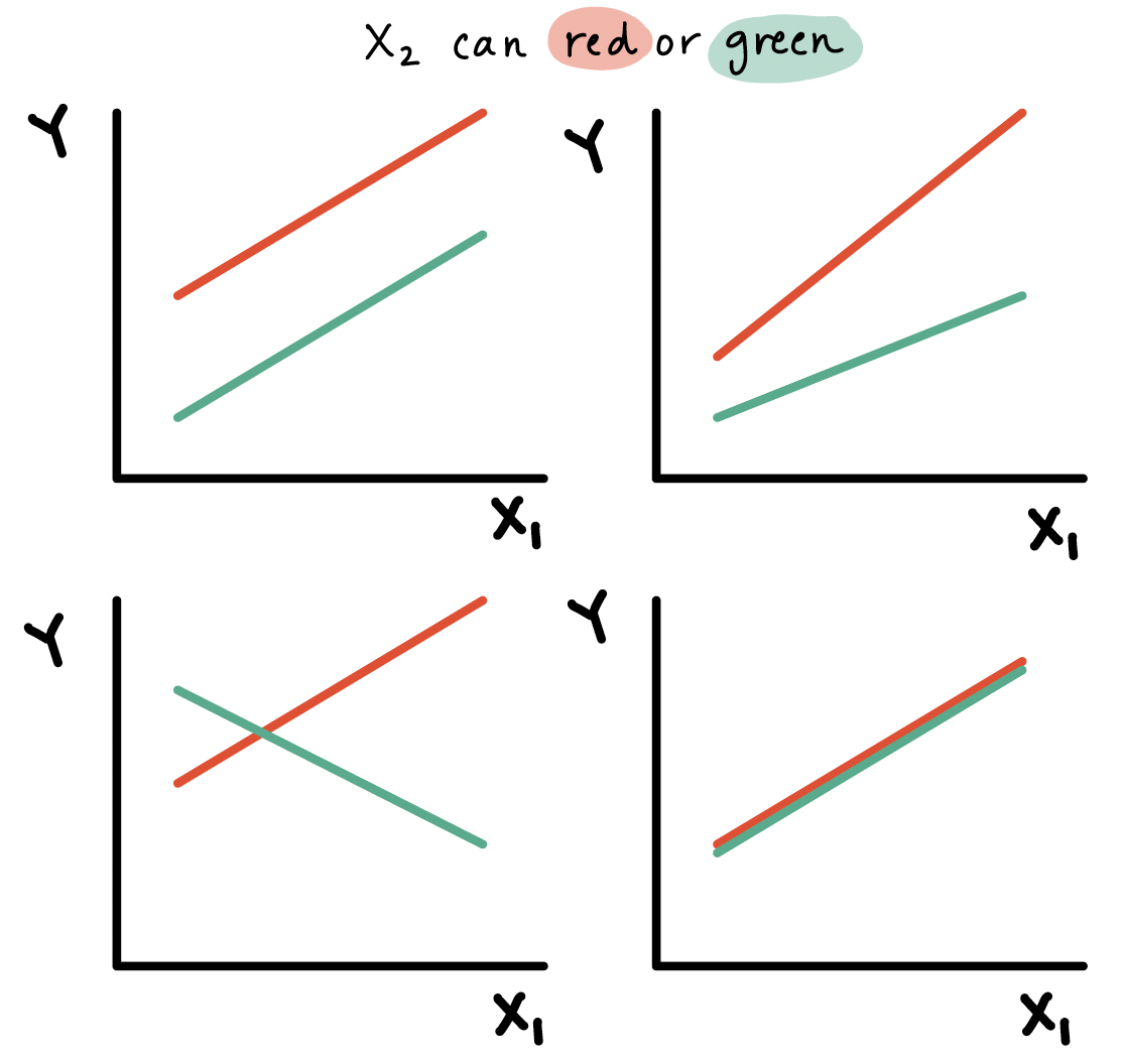
Types of interactions / non-interactions
Common types of interactions:
Synergism: \(X_{2}\) strengthens the \(X_{1}\) effect
Antagonism:\(X_{2}\) weakens the \(X_{1}\) effect
If the interaction coefficient is not significant
- No evidence of effect modification, i.e., the effect of \(X_{1}\) does not vary with \(X_{2}\)
If the main effect of \(X_2\) is also not significant
- No evidence that \(X_2\) is a confounder
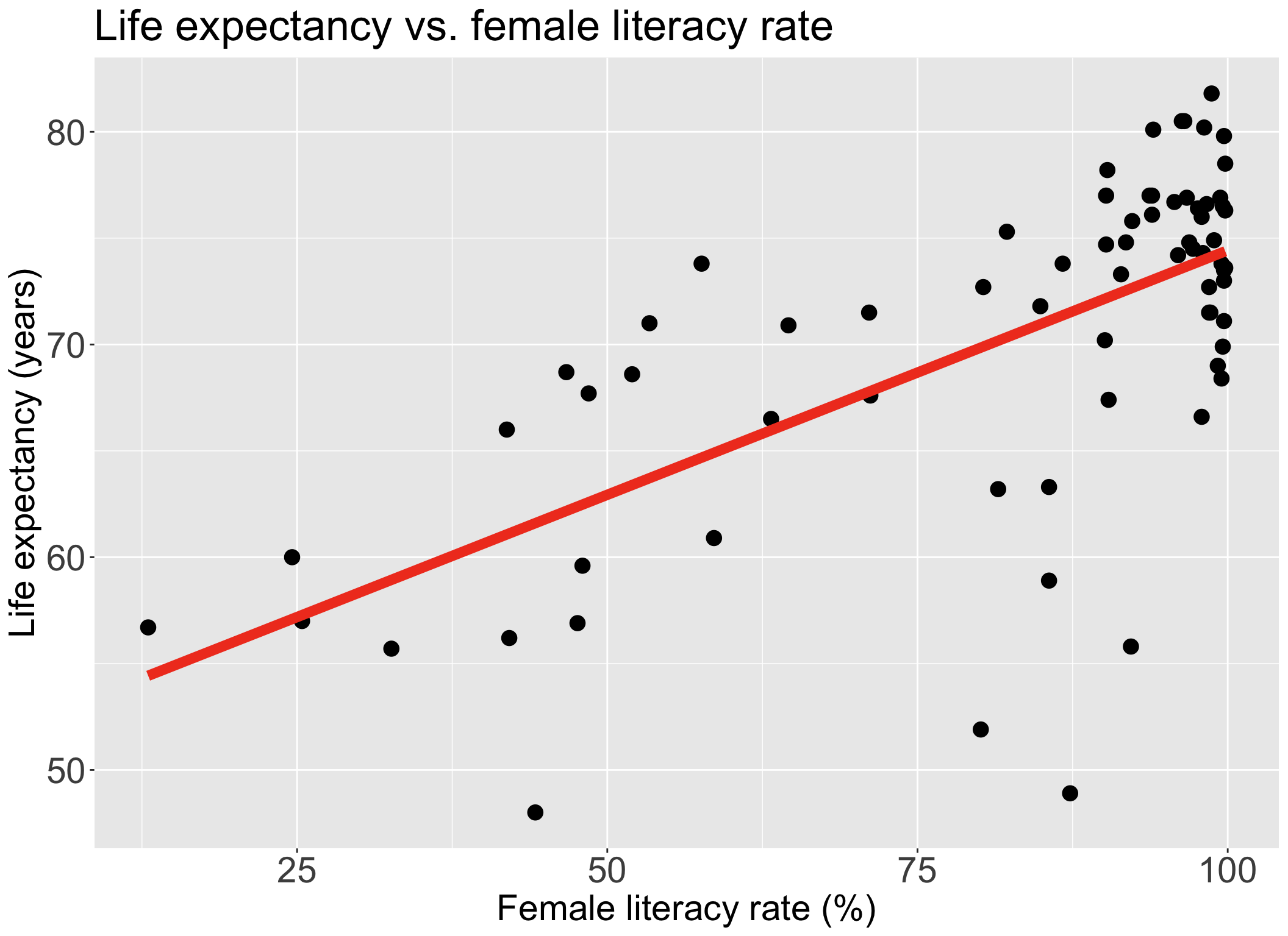
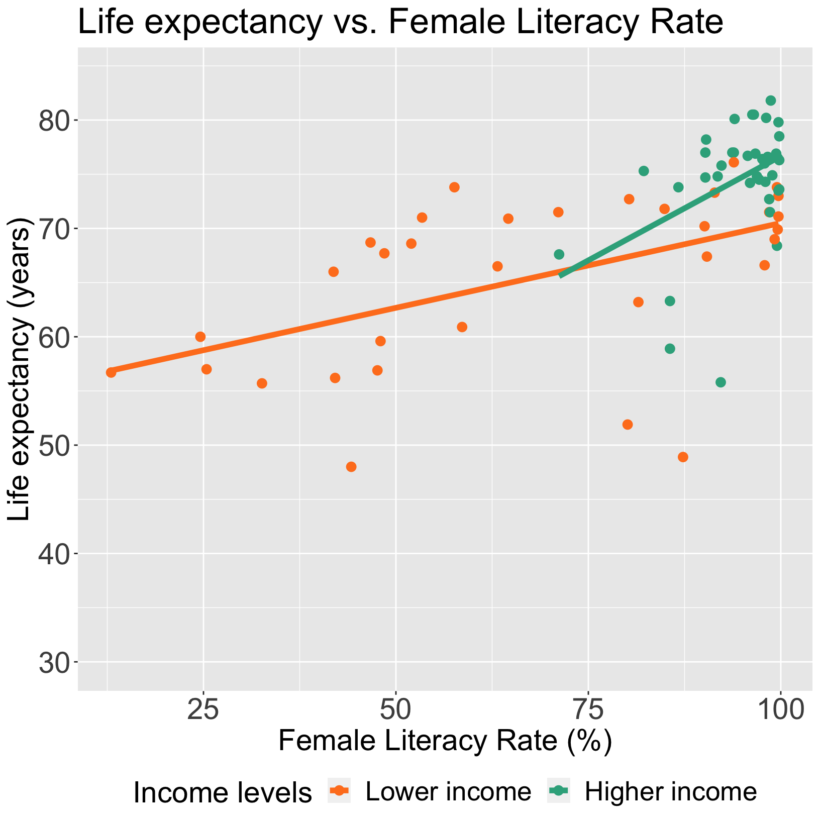
Do we think income level is an effect modifier for female literacy rate?
Let’s say we only have two income groups: low income and high income
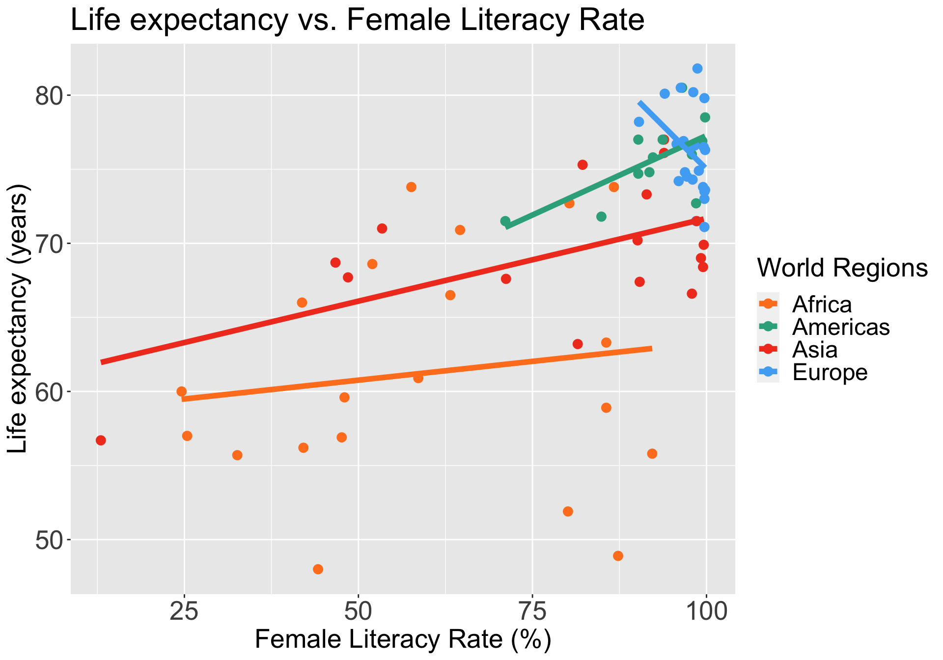
We can start by visualizing the relationship between life expectancy and female literacy rate by income level
Questions of interest: Is the effect of female literacy rate on life expectancy differ depending on income level?
- This is the same as: Is income level is an effect modifier for female literacy rate?
- Let’s run an interaction model to see!
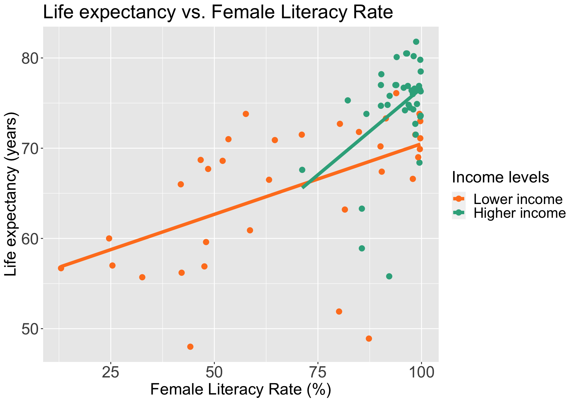
Let’s take a look back at the plot
For lower income countries: \(I(\text{high income}) =0\)
\[ \begin{aligned} \widehat{LE} = & \widehat\beta_0 + \widehat\beta_1 FLR \\ \widehat{LE} = & 54.85 + 0.156 \cdot FLR\\ \end{aligned}\]
For higher income countries: \(I(\text{high income}) =1\)
\[ \begin{aligned} \widehat{LE} = & (\widehat\beta_0 +\widehat\beta_2) + (\widehat\beta_1 +\widehat\beta_3) FLR \\ \widehat{LE} = & (54.85 - 16.65) + (0.156 + 0.228) \cdot FLR\\ \widehat{LE} = & 38.2 + 0.384 \cdot FLR\\ \end{aligned}\]
Do we think world region is an effect modifier for female literacy rate?
We can start by visualizing the relationship between life expectancy and female literacy rate by world region
Questions of interest: Does the effect of female literacy rate on life expectancy differ depending on world region?
- This is the same as: Is world region is an effect modifier for female literacy rate?
Let’s run an interaction model to see!
Centering continuous variables when we are including interactions

- For Europe, the mean life expectancy had a regression line with a large intercept
\[\begin{aligned} \widehat{LE} = &\big(\widehat\beta_0+\widehat\beta_4\big) + \big(\widehat\beta_1 + \widehat\beta_7\big)FLR \\ \widehat{LE} = & (58.23 + 63.63) + (0.051 - 0.519)FLR \\ \widehat{LE} = & 121.86 -0.468FLR \\ \end{aligned}\]
Centering the continuous variables in a model (when they are involved in interactions) helps with:
Interpretations of the coefficient estimates
Correlation between the main effect for the variable and the interaction that it is involved with
- To be discussed in future lecture: leads to multicollinearity issues
Other online sources about when and when not to center:
It’ll be helpful to center female literacy rate
- Centering female literacy rate: \[ FLR^c = FLR - \overline{FLR}\]
- Centering in R:
- I’m going to print the mean so I can use it for my interpretations
Now all intercept values (in each respective world region) will be the mean life expectancy when female literacy rate is 82.03%
We will used center FLR for the rest of the lecture
Now we refit the model with the centered FLR
m_int_wr_flrc = lm(LifeExpectancyYrs ~ FLR_c*four_regions,
                data = gapm_sub)
tidy(m_int_wr_flrc, conf.int=T) %>% gt() %>% tab_options(table.font.size = 35) %>% fmt_number(decimals = 3)| term | estimate | std.error | statistic | p.value | conf.low | conf.high |
|---|---|---|---|---|---|---|
| (Intercept) | 62.387 | 1.626 | 38.358 | 0.000 | 59.138 | 65.637 |
| FLR_c | 0.051 | 0.053 | 0.957 | 0.342 | −0.055 | 0.157 |
| four_regionsAmericas | 11.032 | 2.918 | 3.781 | 0.000 | 5.203 | 16.862 |
| four_regionsAsia | 7.287 | 2.042 | 3.568 | 0.001 | 3.207 | 11.367 |
| four_regionsEurope | 21.038 | 7.698 | 2.733 | 0.008 | 5.659 | 36.417 |
| FLR_c:four_regionsAmericas | 0.164 | 0.197 | 0.830 | 0.410 | −0.231 | 0.558 |
| FLR_c:four_regionsAsia | 0.061 | 0.073 | 0.830 | 0.410 | −0.086 | 0.208 |
| FLR_c:four_regionsEurope | −0.519 | 0.476 | −1.090 | 0.280 | −1.471 | 0.432 |
- What changed? What stayed the same? What’s the new intercept for Europe?
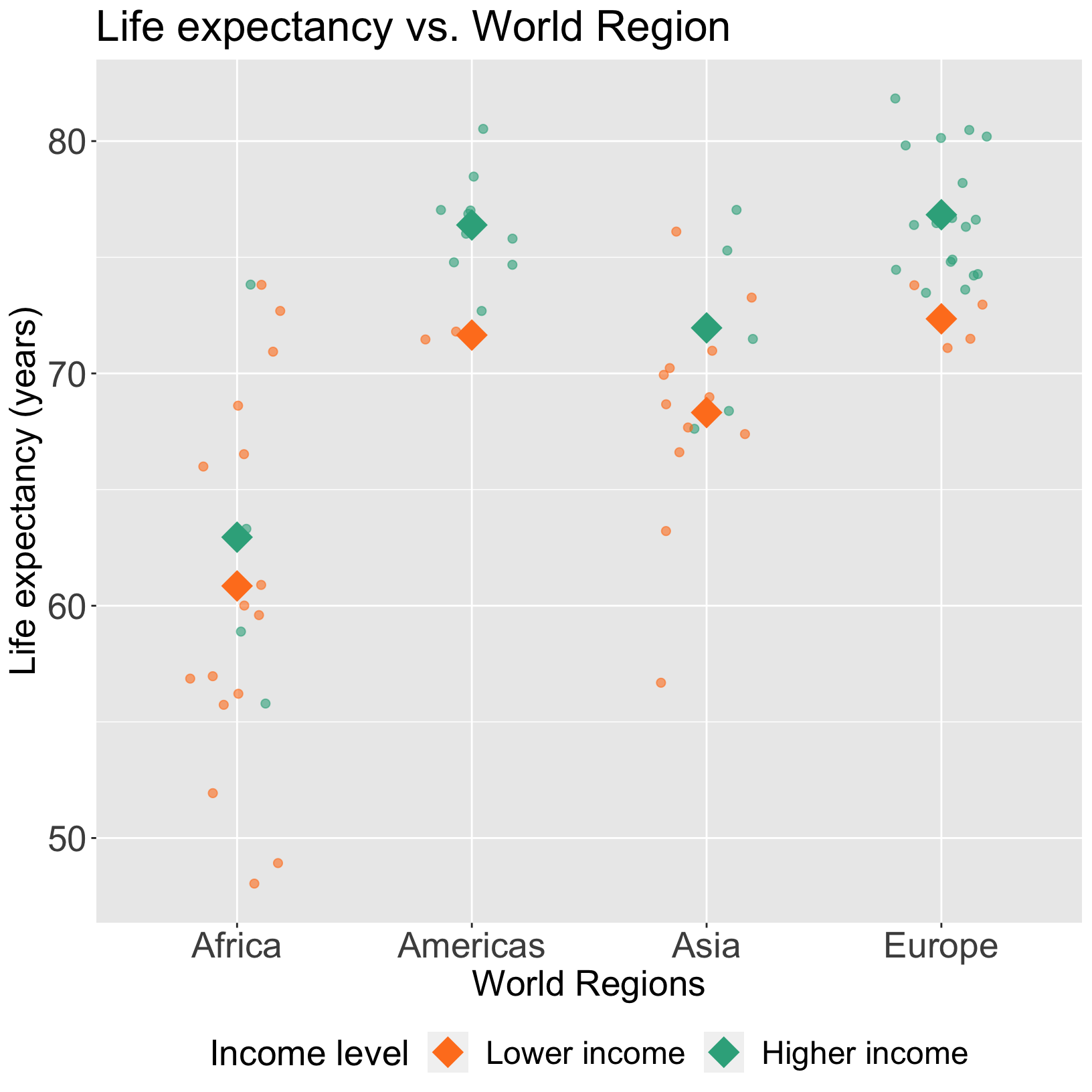
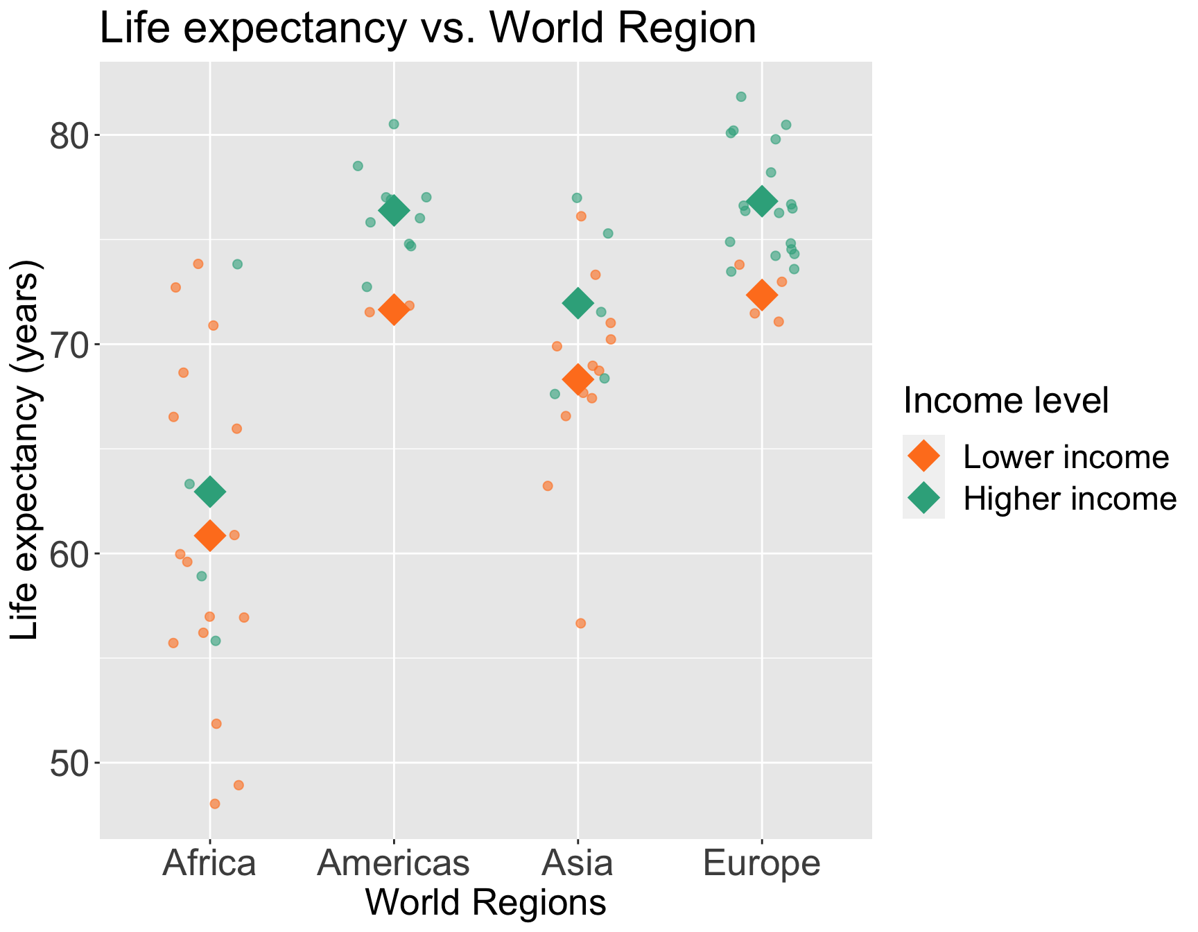
Do we think income level can be an effect modifier for world region?
Taking a break from female literacy rate to demonstrate interactions for two categorical variables
We can start by visualizing the relationship between life expectancy and world region by income level
Questions of interest: Does the effect of world region on life expectancy differ depending on income level?
- This is the same as: Is income level an effect modifier for world region?
Let’s run an interaction model to see!
Poll Everywhere Question 4
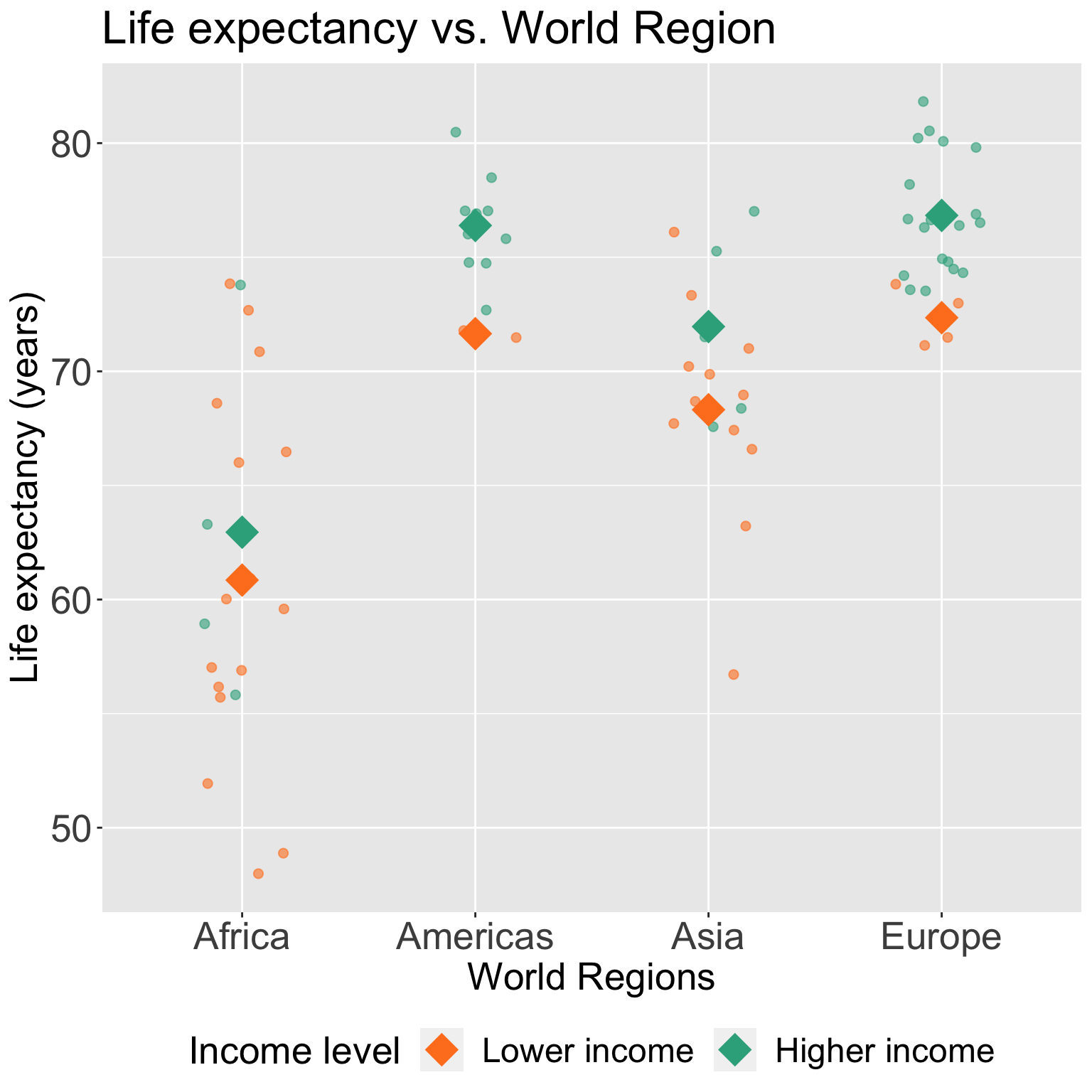
Let’s take a look back at the plot
For lower income countries: \(I(\text{high income}) =0\)
\[ \begin{aligned} \widehat{LE} = &\widehat\beta_0 + \widehat\beta_2 I(\text{Americas}) + \widehat\beta_3 I(\text{Asia}) + \\ & \widehat\beta_4 I(\text{Europe}) \\ \end{aligned}\]
For higher income countries: \(I(\text{high income}) =1\)
\[ \begin{aligned} \widehat{LE} = & (\widehat\beta_0 + \widehat\beta_1) + (\widehat\beta_2 + \widehat\beta_5) I(\text{Americas}) + \\& (\widehat\beta_3 + \widehat\beta_6) I(\text{Asia}) + (\widehat\beta_4 + \widehat\beta_7) I(\text{Europe}) \\ \end{aligned}\]