R09: Summarizing data with `tidyverse`

Author

Nicky Wakim

Published

December 4, 2024

Where are we?

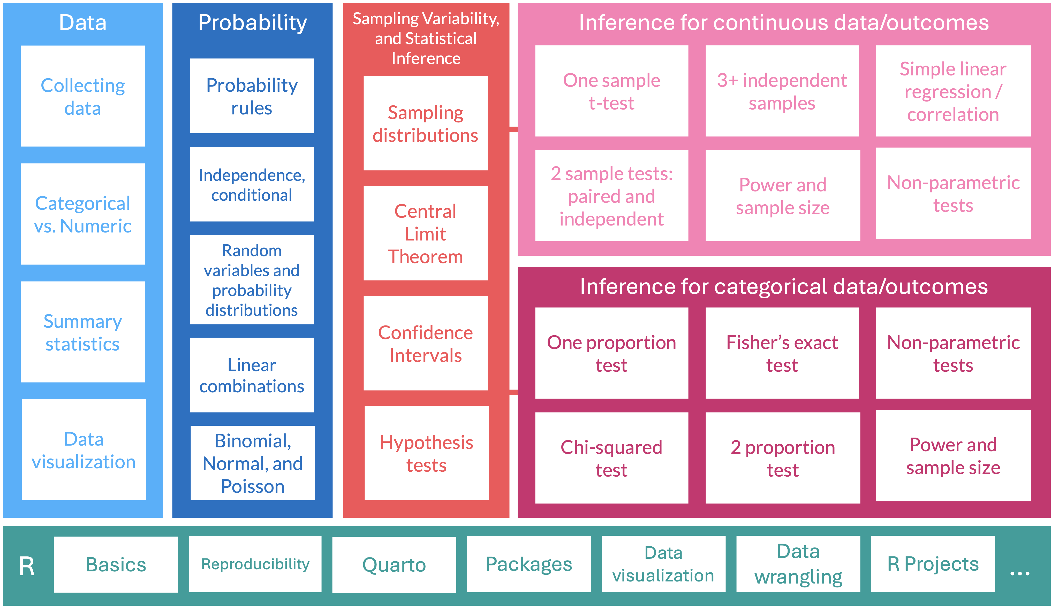
What is the tidyverse? (revisited)

The tidyverse is a collection of R packages designed for data science. All packages share an underlying design philosophy, grammar, and data structures.

ggplot2 - data visualisation
dplyr - data manipulation
tidyr - tidy data
readr - read rectangular data
purrr - functional programming
tibble - modern data frames
stringr - string manipulation
forcats - factors
and many more …

Tidy data¹

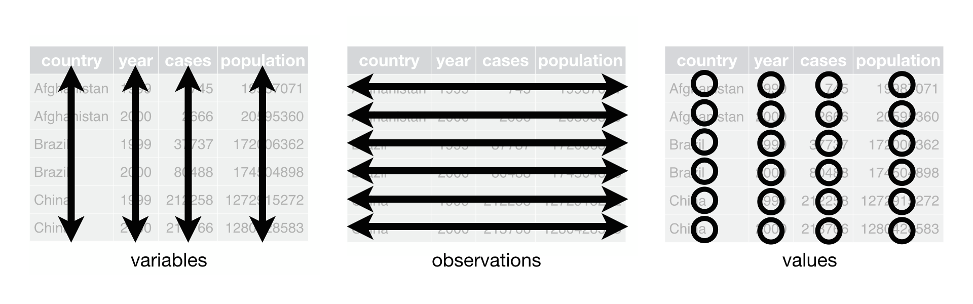
Each variable must have its own column.
Each observation must have its own row.
Each value must have its own cell.

Pipe operator (`magrittr`)

The pipe operator (%>%) allows us to step through sequential functions in the same way we follow if-then statements or steps from instructions

I want to find my keys, then start my car, then drive to work, then park my car.

Nested

park(drive(start_car(find("keys")), 
           to = "work"))

Piped

find("keys") %>%
  start_car() %>%
  drive(to = "work") %>%
  park()

Using `summarize()`

`group_by()`: group by one or more variables

What if I want to quickly look at group differences?
It will not change how the data look, but changes the actions of following functions

I want to group my data by sex assigned at birth.

dds.discr5 = dds.discr2 %>%
  group_by(SAB)
glimpse(dds.discr5)

Rows: 1,000
Columns: 7
Groups: SAB [2]
$ id           <int> 10210, 10409, 10486, 10538, 10568, 10690, 10711, 10778, 1…
$ age.cohort   <fct> 13-17, 22-50, 0-5, 18-21, 13-17, 13-17, 13-17, 13-17, 13-…
$ age          <int> 17, 37, 3, 19, 13, 15, 13, 17, 14, 13, 13, 14, 15, 17, 20…
$ SAB          <fct> Female, Male, Male, Female, Male, Female, Female, Male, F…
$ expenditures <int> 2113, 41924, 1454, 6400, 4412, 4566, 3915, 3873, 5021, 28…
$ R_E          <fct> White not Hispanic, White not Hispanic, Hispanic, Hispani…
$ exp_to_age   <dbl> 124.2941, 1133.0811, 484.6667, 336.8421, 339.3846, 304.40…

Let’s see how the groups change something like the summarize() function in the next slide

`summarize()`: summarize your data or grouped data into one row

What if I want to calculate specific descriptive statistics for my variables?
This function is often best used with group_by()
If only presenting the summaries, functions like tbl_summary() is better
summarize() creates a new data frame, which means you can plot and manipulate the summarized data

Over whole sample:

dds.discr2 %>% 
  summarize(
    ave = mean(expenditures),
    SD = sd(expenditures),
    med = median(expenditures))

# A tibble: 1 × 3
     ave     SD   med
   <dbl>  <dbl> <dbl>
1 18066. 19543.  7026

Grouped by sex assigned at birth:

dds.discr2 %>% 
  group_by(SAB) %>% 
  summarize(
    ave = mean(expenditures),
    SD = sd(expenditures),
    med = median(expenditures))

# A tibble: 2 × 4
  SAB       ave     SD   med
  <fct>   <dbl>  <dbl> <int>
1 Female 18130. 20020.  6400
2 Male   18001. 19068.  7219

Using `get_summary_stats()`

`get_summary_stats()` from `rstatix` package

dds.discr2 %>% get_summary_stats()

# A tibble: 4 × 13
  variable     n    min   max median     q1     q3    iqr    mad    mean      sd
  <fct>    <dbl>  <dbl> <dbl>  <dbl>  <dbl>  <dbl>  <dbl>  <dbl>   <dbl>   <dbl>
1 id        1000 1.02e4 99898 55384. 31809. 76135. 44326  3.27e4 54663.  25644. 
2 age       1000 0         95    18     12     26     14  1.04e1    22.8    18.5
3 expendi…  1000 2.22e2 75098  7026   2899. 37713. 34814  7.76e3 18066.  19543. 
4 exp_to_…  1000 2.76e1   Inf   462.   274.   938.   664. 3.54e2   Inf     NaN  
# ℹ 2 more variables: se <dbl>, ci <dbl>

dds.discr2 %>% 
  group_by(R_E) %>%
  get_summary_stats(expenditures, type = "common")

# A tibble: 8 × 11
  R_E       variable     n   min   max median    iqr   mean     sd     se     ci
  <fct>     <fct>    <dbl> <dbl> <dbl>  <dbl>  <dbl>  <dbl>  <dbl>  <dbl>  <dbl>
1 American… expendi…     4  3726 58392 41818. 34085. 36438. 25694. 12847. 40885.
2 Asian     expendi…   129   374 75098  9369  30892  18392. 19209.  1691.  3346.
3 Black     expendi…    59   240 60808  8687  37987  20885. 20549.  2675.  5355.
4 Hispanic  expendi…   376   222 65581  3952   7961. 11066. 15630.   806.  1585.
5 Multi Ra… expendi…    26   669 38619  2622   2060.  4457.  7332.  1438.  2962.
6 Native H… expendi…     3 37479 50141 40727   6331  42782.  6576.  3797. 16337.
7 Other     expendi…     2  2018  4615  3316.  1298.  3316.  1836.  1298. 16499.
8 White no… expendi…   401   340 68890 15718  39157  24698. 20604.  1029.  2023.

How to force all output to be shown? (1/2)

Use kable() from the knitr package.

dds.discr2 %>% get_summary_stats() %>% kable()

variable	n	min	max	median	q1	q3	iqr	mad	mean	sd	se	ci
id	1000	10210.000	99898	55384.500	31808.750	76134.750	44326.000	32734.325	54662.85	25643.673	810.924	1591.310
age	1000	0.000	95	18.000	12.000	26.000	14.000	10.378	22.80	18.462	0.584	1.146
expenditures	1000	222.000	75098	7026.000	2898.750	37712.750	34814.000	7760.670	18065.79	19542.831	617.999	1212.724
exp_to_age	1000	27.571	Inf	461.752	273.881	938.125	664.244	353.971	Inf	NaN	NaN	NaN

How to force all output to be shown? `knitr` (2/2)

Use kable() from the knitr package.

dds.discr2 %>% 
  group_by(R_E) %>%
  get_summary_stats(expenditures, type = "common") %>% 
  kable()

R_E	variable	n	min	max	median	iqr	mean	sd	se	ci
American Indian	expenditures	4	3726	58392	41817.5	34085.25	36438.250	25693.912	12846.956	40884.748
Asian	expenditures	129	374	75098	9369.0	30892.00	18392.372	19209.225	1691.278	3346.482
Black	expenditures	59	240	60808	8687.0	37987.00	20884.593	20549.274	2675.288	5355.170
Hispanic	expenditures	376	222	65581	3952.0	7961.25	11065.569	15629.847	806.048	1584.940
Multi Race	expenditures	26	669	38619	2622.0	2059.75	4456.731	7332.135	1437.950	2961.514
Native Hawaiian	expenditures	3	37479	50141	40727.0	6331.00	42782.333	6576.462	3796.922	16336.838
Other	expenditures	2	2018	4615	3316.5	1298.50	3316.500	1836.356	1298.500	16499.007
White not Hispanic	expenditures	401	340	68890	15718.0	39157.00	24697.549	20604.376	1028.933	2022.793

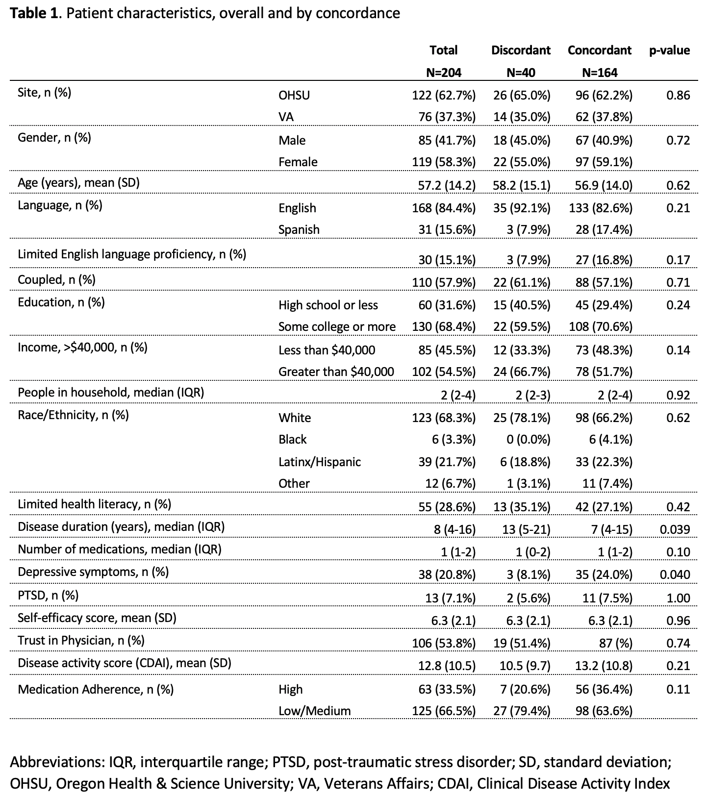
Making a Table 1

Table 1 example

Often, research studies will show a table with all the summary statistics (lovingly called “Table 1”)
Basic Table 1 will show all variables with:
- Mean and SD for the numeric variables
- \(n (\%)\) for categorical variables

Are We on the Same Page?: A Cross-Sectional Study of Patient-Clinician Goal Concordance in Rheumatoid Arthritis
J Barton et al.
Arthritis Care & Research.
2021 Sep 27 https://pubmed.ncbi.nlm.nih.gov/34569172/

`tbl_summary()` : table summary (1/2)

What if I want one of those fancy summary tables that are at the top of most research articles?

library(gtsummary)
tbl_summary(dds.discr2)

Characteristic	N = 1,000¹
id	55,385 (31,759, 76,205)
age.cohort
0-5	82 (8.2%)
6-12	175 (18%)
13-17	212 (21%)
18-21	199 (20%)
22-50	226 (23%)
51+	106 (11%)
age	18 (12, 26)
SAB
Female	503 (50%)
Male	497 (50%)
expenditures	7,026 (2,898, 37,718)
R_E
American Indian	4 (0.4%)
Asian	129 (13%)
Black	59 (5.9%)
Hispanic	376 (38%)
Multi Race	26 (2.6%)
Native Hawaiian	3 (0.3%)
Other	2 (0.2%)
White not Hispanic	401 (40%)
exp_to_age	462 (273, 938)
¹ Median (Q1, Q3); n (%)

`tbl_summary()` : table summary (2/2)

Let’s make this more presentable

dds.discr2 %>%
  select(-id, -age.cohort, -exp_to_age) %>%
  tbl_summary(label = c(age ~ "Age", 
                        R_E ~ "Race/Ethnicity", 
                        SAB ~ "Sex Assigned at Birth", 
                        expenditures ~ "Expenditures"),
              statistic = list(all_continuous() ~ 
                                 "{mean} ({sd})"))

Characteristic	N = 1,000¹
Age	23 (18)
Sex Assigned at Birth
Female	503 (50%)
Male	497 (50%)
Expenditures	18,066 (19,543)
Race/Ethnicity
American Indian	4 (0.4%)
Asian	129 (13%)
Black	59 (5.9%)
Hispanic	376 (38%)
Multi Race	26 (2.6%)
Native Hawaiian	3 (0.3%)
Other	2 (0.2%)
White not Hispanic	401 (40%)
¹ Mean (SD); n (%)

Resources

`dplyr` resources

More dpylr functions to reference!

Additional details and examples are available in the vignettes:

and the dplyr 1.0.0 release blog posts:

R programming class at OHSU!

You can check out Dr. Jessica Minnier’s R class page if you want more notes, videos, etc.

The larger tidy ecosystem

Just to name a few…

Credit to Mine Çetinkaya-Rundel

These notes were built from Mine’s notes
- Most pages and code were left as she made them
- I changed a few things to match our class
Please see her Github repository for the original notes

Footnotes

Source: R for Data Science. Grolemund and Wickham.↩︎

Where are we?

What is the tidyverse? (revisited)

Tidy data1

Pipe operator (magrittr)

Using summarize()

group_by(): group by one or more variables

summarize(): summarize your data or grouped data into one row

Using get_summary_stats()

get_summary_stats() from rstatix package