Lesson 13: Model Diagnostics

Nicky Wakim

2026-05-11

Learning Objectives

  1. Understand the components of calculations for logistic regression diagnostics

  2. Plot and determine observations where regression does not fit well or are influential using specific diagnostic values

Review of model assessment so far

  • Overall measurements of fit

    • How well does the fitted logistic regression model predict the outcome?

    • Different ways to measure the answer to this question

Measure of fit Hypothesis tested? Equation R code
Pearson residual Yes \(X^2=\sum_{j=1}^{J}{r\left(Y_j,{\widehat{\pi}}_j\right)^2}\) Not given
Hosmer-Lemeshow test Yes \(\widehat{C}=\sum_{k=1}^{g}\frac{\left(o_k-n_k^\prime{\bar{\pi}}_k\right)^2}{n_k^\prime{\bar{\pi}}_k(1-{\bar{\pi}}_k)}\) hoslem.test()
AUC-ROC Kinda Not given auc(observed, predicted)
AIC Only to compare models \(AIC = -2 \cdot \text{log-likelihood} + 2q\) AIC(model_name)
BIC Only to compare models \(BIC = -2 \cdot \text{log-likelihood} + q\text{log}(n)\) BIC(model_name)

Next week for model assessment

  • Numerical problems

    • Assess pre and post model fit
    • Numerical problems often depend on the final model (which variables and interactions are included)


  • Different numerical problems to look out for

    • Zero cell count
    • Complete separation
    • Multicollinearity


  • Today: We now use model diagnostics to identify any observations that the model does not fit well

Assumptions: Linear Regression vs. Logistic Regression

Linear Regression Assumptions

  • Linearity of relationship between \(Y\) and covariates
  • Independence of observations
  • Normality of \(Y\) given \(X\) (residuals)
  • Equality of variance of residuals (homoscedasticity)

Logistic Regression Assumptions

  • Linearity of relationship between logit of outcome and covariates
  • Independence of observations
  • Distribution of \(Y\) given \(X\) follows the prescribed one (binomial in our case)
  • Back in Lesson 5: Simple Logistic Regression, we walk through linear regression assumptions that do not hold for logistic regression
  • Because our assumptions for logistic regression are a little different than linear regression, we need slightly different diagnostic tools to assess observations that may be outliers or influential points

Learning Objectives

  1. Understand the components of calculations for logistic regression diagnostics
  1. Plot and determine observations where regression does not fit well or are influential using specific diagnostic values

(Some) Diagnostics of Logistic Regression

  • Measures at the observation level for model diagnostics!

  • Model diagnostics of logistic regression can be assessed by checking for outliers:

      1. Standardized Deviance residuals, \(d_i\)


  • Model diagnostics of logistic regression can be assessed by checking how influential an observation is:

      1. Cook’s distance, \(D_i\)
      1. Change in coefficients, \(DFBETA\) or \(\Delta \widehat{\beta}_j\)
      1. Change in estimated probabilities, \(DFFITS_i\)

1. Standardized Deviance Residuals (\(d_i\))

  • Identifies outliers: observations where the model’s prediction is far from the truth.

\[\text{deviance residual}_i = \text{sign}(y_i - \widehat{\pi}_i) \cdot \sqrt{-2\left[y_i\log\left(\dfrac{y_i}{\widehat{\pi}_i}\right) + (1-y_i)\log\left(\dfrac{1-y_i}{1-\widehat{\pi}_i}\right)\right]}\]

  • Standardized to account for leverage (\(h_i\), measure of distance between observed predictors and mean predictors):

\[d_i = \frac{\text{deviance residual}_i}{\sqrt{1-h_i}}\]

  • Rule of Thumb: Large values (typically \(|d_i| > 3\)) indicate that the model does not fit observation \(i\) well

2. Cook’s Distance (\(D_i\))

  • Measures the aggregate influence of an observation on all regression coefficients.
  • It asks: “How much would the whole model change if we deleted this pattern?”
  • Combined measure of leverage (\(h_i\)) and the residual, with \(k\) coefficients.

\[D_i = \dfrac{d_i^2 h_i}{(k-1)(1-h_i)^2}\]

  • Rule of Thumb: Flag values where \(D_i > 1\) or \(D_i > 4/n\)

3. Change in Coefficients (DFBETA)

  • Measures the change in a specific coefficient \(\widehat{\beta}_j\) if an observation is excluded.

\[\Delta \widehat{\beta}_j = \frac{\widehat{\beta}_j - \widehat{\beta}_{j(-i)}}{SE(\widehat{\beta}_{j(-i)})}\]

  • Useful for ensuring our variable of interest (e.g., Prior Fracture) isn’t being driven by a single observation
  • This is different than the change in coefficient when we remove a predictor from the model (e.g., change in coefficient for prior fracture when we remove age from the model)
  • Rule of Thumb: Look for \(|DFBETA| > \dfrac{2}{\sqrt{n}}\).

4. Change in fitted probabilities (DFFITS)

  • Measures the impact on the predicted probability (the “fit”)

  • It is the number of standard deviations the fitted value changes when an observation is removed

  • Rule of Thumb: Flag if \(|DFFITS| > 2\sqrt{k/n}\)

Learning Objectives

  1. Understand the components of calculations for logistic regression diagnostics
  1. Plot and determine observations where regression does not fit well or are influential using specific diagnostic values

Recall the model we fit: GLOW Study with interactions

  • Outcome variable: any fracture in the first year of follow up (FRACTURE: 0 or 1)

  • Risk factor/variable of interest: history of prior fracture (PRIORFRAC: 0 or 1)

  • Potential confounder or effect modifier: age (AGE, a continuous variable)

  • Fitted model with interactions: \[\begin{aligned} \text{logit}\left(\widehat\pi(\mathbf{X})\right) & = \widehat\beta_0 &+ &\widehat\beta_1\cdot I(\text{PF}) & + &\widehat\beta_2\cdot Age& + &\widehat\beta_3 \cdot I(\text{PF}) \cdot Age \\ \text{logit}\left(\widehat\pi(\mathbf{X})\right) & = -1.376 &+ &1.002\cdot I(\text{PF})& + &0.063\cdot Age& -&0.057 \cdot I(\text{PF}) \cdot Age \end{aligned}\]


  • Lesson 12: determined the overall fit of this model
  • Today: determine the if any observations/covariate patterns that model does not fit well

Recall our friend augment()?

# Augment for residuals
library(broom)
aug_glow = augment(glow_m3, type.predict = "response", type.residuals = "deviance")

# Calculate influence measures (Cook's D, DFFITS, DFBETAs)
infl = influence.measures(glow_m3)
dx_glow = cbind(aug_glow, as.data.frame(infl$infmat)) %>%
          dplyr::select(-c(cook.d, cov.r, hat))

Key to the values

  • .fitted: Estimated probability of events (\(\widehat{\pi}\))
  • .resid: Deviance residual
  • .hat: Leverage
  • .sigma: Standard error of the residuals
  • .cooksd: Cook’s distance
  • .std.resid: Standardized deviance residual
  • dfb.1_: Change in coef. estimate for intercept
  • dfb.prrY: Change in coef. estimate for prior fracture
  • dfb.age_c: Change in coef. estimate for age
  • dfb.pY:_: Change in coef. estimate for interaction between age and prior fracture
  • dffit: Change in predicted probability of fracture
glimpse(dx_glow, width=50)
Rows: 500
Columns: 14
$ fracture   <fct> No, No, No, No, No, No, No, N…
$ priorfrac  <fct> No, No, Yes, No, No, Yes, No,…
$ age_c      <dbl> -7, -4, 19, 13, -8, -2, 15, 1…
$ .fitted    <dbl> 0.1402159, 0.1643855, 0.43133…
$ .resid     <dbl> -0.5496799, -0.5993128, -1.06…
$ .hat       <dbl> 0.003811004, 0.003143864, 0.0…
$ .sigma     <dbl> 1.027863, 1.027807, 1.027018,…
$ .cooksd    <dbl> 0.0001565683, 0.0001555953, 0…
$ .std.resid <dbl> -0.5507303, -0.6002571, -1.07…
$ dfb.1_     <dbl> -2.632841e-02, -2.994570e-02,…
$ dfb.prrY   <dbl> 0.01472703, 0.01675039, -0.01…
$ dfb.ag_c   <dbl> 2.185329e-02, 1.536230e-02, -…
$ `dfb.pY:_` <dbl> -0.013507094, -0.009495139, -…
$ dffit      <dbl> -0.03314002, -0.03279756, -0.…

Cutoffs and visual assessment for diagnostics

  • The plots allow us to identify those covariate patterns that are…

    • Poorly fit

      • Large values of standardized deviance residuals (\(d_i\))
    • Influential on estimated coefficients

      • Large values of Cook’s distance (\(D_i\)), change in coefficient estimates (\(\Delta \widehat{\beta}_j\)), and change in predicted probabilities (\(DFFITS_i\))
  • We plot the diagnostic values against the predicted probabilities to see if there are any patterns in the poorly fit or influential observations

GLOW Study: Standardized Deviance Residuals

  • Look for \(|d_i| > 3\)
  • Points at the top/bottom indicate patterns where \(Y\) is the opposite of what we expected
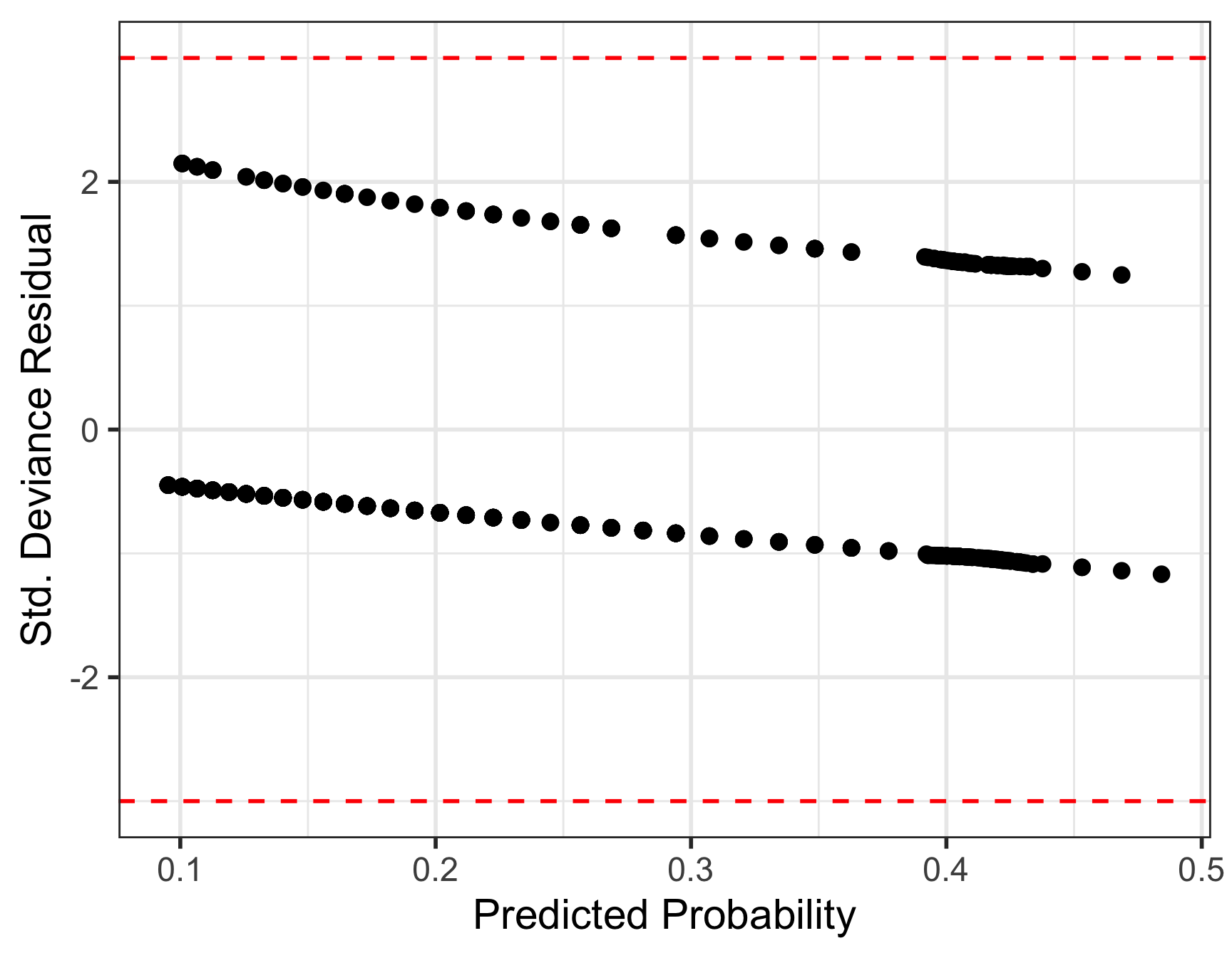
dx_glow %>% filter(abs(.std.resid) > 3) |> 
  dplyr::select(priorfrac, age_c, 
                .fitted, .std.resid)
[1] priorfrac  age_c      .fitted    .std.resid
<0 rows> (or 0-length row.names)
Code
ggplot(dx_glow, aes(x = .fitted, y = .std.resid)) +
  geom_point() +
  geom_hline(yintercept = c(-3, 3), col = "red", linetype="dashed") +
  labs(x = "Predicted Probability", y = "Std. Deviance Residual")

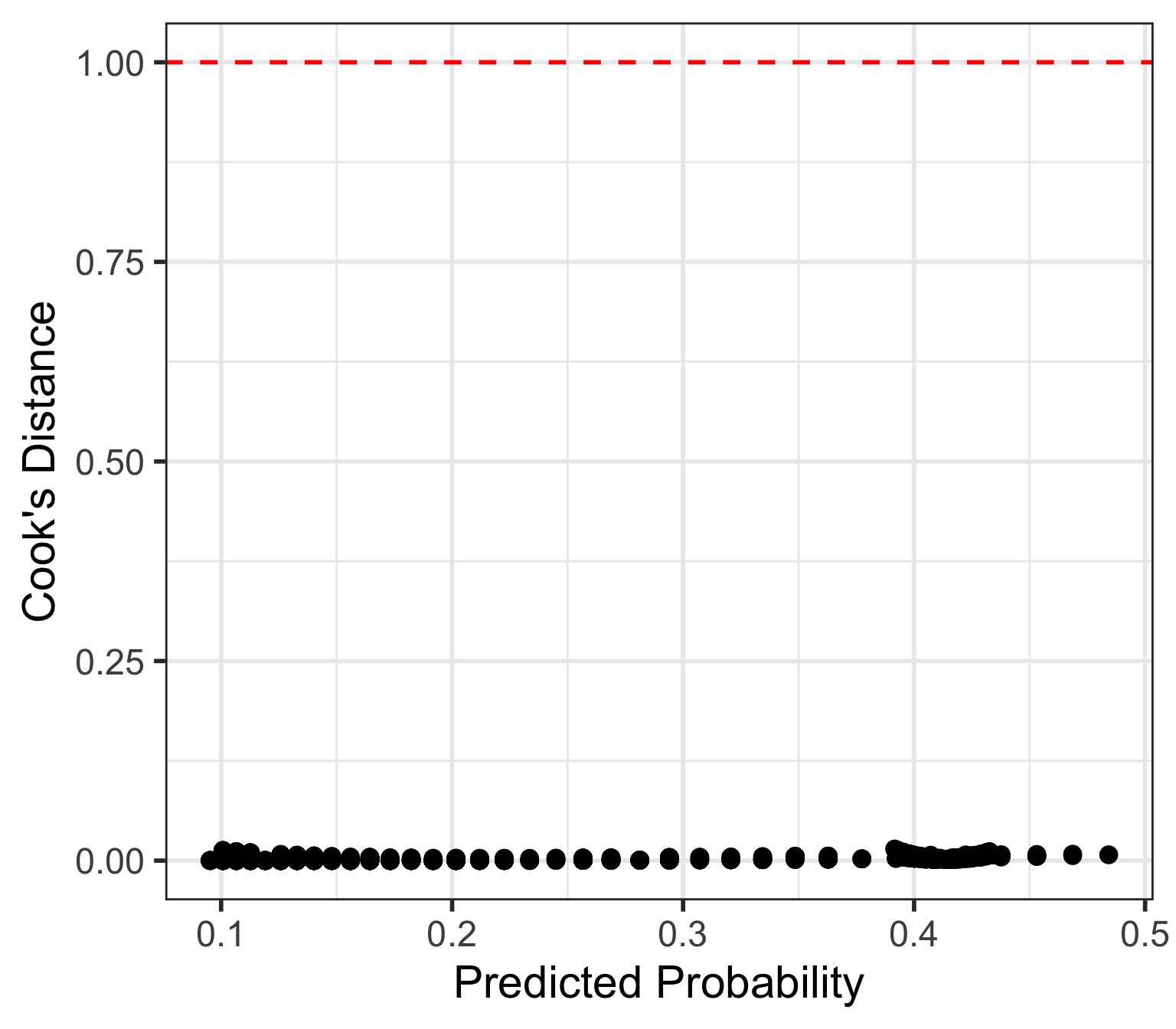
GLOW Study: Cook’s Distance

  • Threshold: \(D_i > 1\)
  • Points above the line are influential on our results.
dx_glow %>% filter(.cooksd > 1) %>%
  dplyr::select(priorfrac, age_c, .fitted, .cooksd)
[1] priorfrac age_c     .fitted   .cooksd  
<0 rows> (or 0-length row.names)
Code
ggplot(dx_glow, aes(x = .fitted, y = .cooksd)) +
  geom_point() +
  geom_hline(yintercept = 1, col = "red", linetype="dashed") +
  labs(x = "Predicted Probability", y = "Cook's Distance")

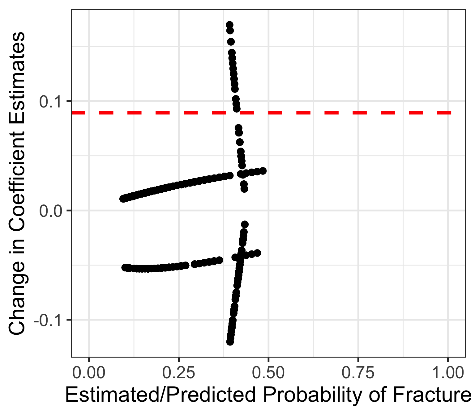
GLOW Study: Change in coefficient estimates (for prior fracture)

  • Book recommends flagging observsations if change in coefficient estimates are greater than \(2/\sqrt{n}\)
dx_glow %>% filter(dfb.prrY > 2/sqrt(500)) %>% 
  select(priorfrac, age_c, .fitted, dfb.prrY) %>%
  head(15)
    priorfrac age_c   .fitted   dfb.prrY
377       Yes     3 0.4113188 0.09307664
383       Yes    -8 0.3977192 0.14436585
385       Yes     3 0.4113188 0.09307664
387       Yes     1 0.4088354 0.10203872
404       Yes    -7 0.3989493 0.13946650
409       Yes    -3 0.4038826 0.12039584
411       Yes    -2 0.4051190 0.11574619
412       Yes    -4 0.4026474 0.12509002
415       Yes    -6 0.4001808 0.13462262
417       Yes    -1 0.4063566 0.11113848
422       Yes    -2 0.4051190 0.11574619
429       Yes    -7 0.3989493 0.13946650
436       Yes    -4 0.4026474 0.12509002
444       Yes    -7 0.3989493 0.13946650
453       Yes     1 0.4088354 0.10203872
To make the plot
ggplot(dx_glow) + 
  geom_hline(yintercept = 2/sqrt(500), col = "red", linetype="dashed", size=2) +
  geom_point(aes(x=.fitted, y=dfb.prrY), size = 3) + 
  xlab("Estimated/Predicted Probability of Fracture") +
  ylab("Change in Coefficient Estimates") +
  theme(text = element_text(size = 26)) + xlim(0,1)

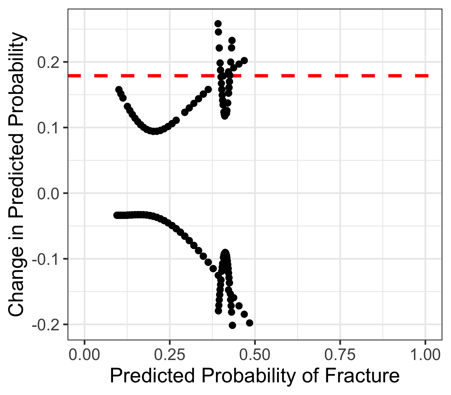
GLOW Study: Changed in predicted probability

  • Flag if \(|DFFITS| > 2\sqrt{k/n}\)
dx_glow %>% filter(abs(dffit) > 2*sqrt(4/500)) %>% 
  select(priorfrac, age_c, .fitted, dffit) %>%
  head(15)
    priorfrac age_c   .fitted      dffit
3         Yes    19 0.4313389 -0.1813034
169       Yes    21 0.4338587 -0.2014239
178        No    20 0.4686423 -0.1845408
192       Yes   -12 0.3928116 -0.1793038
228       Yes   -12 0.3928116 -0.1793038
280        No    21 0.4842350 -0.1977886
328       Yes    21 0.4338587 -0.2014239
383       Yes    -8 0.3977192  0.1983474
398        No    20 0.4686423  0.2020885
404       Yes    -7 0.3989493  0.1875104
408       Yes    20 0.4325984  0.2326503
421       Yes    15 0.4263101  0.1794865
424       Yes    20 0.4325984  0.2326503
429       Yes    -7 0.3989493  0.1875104
444       Yes    -7 0.3989493  0.1875104
To make the plot
ggplot(dx_glow) + 
  geom_hline(yintercept = 2*sqrt(4/500), col = "red", linetype="dashed", size=2) +
  geom_point(aes(x=.fitted, y=dffit), size = 3) + 
  xlab("Predicted Probability of Fracture") +
  ylab("Change in Predicted Probability") +
  theme(text = element_text(size = 26)) + xlim(0,1)

After identifying points

  • Do a data quality check


  • We are not too worried about a few outliers


  • If we have quite a lot of outliers that are highly influential, potential reasons can be considered:

    • The link used in logistic regression model is not appropriate for outcome

      • This is usually unlikely, since logistic regression model is very flexible (think back to why we transformed our outcome from binary form)
    • One or more important covariates missing in the model

      • At least one of the covariates in the model has been entered in the wrong scale (think age-squared vs. age)

How would I report this? (Combining all model assessment)

  • Assuming I have not checked other final models (no other models to compare AIC/BIC or AUC with)

Methods: Our final logistic regression model consisted of the outcome, fracture, and predictors including prior fracture, age, and their interaction. To assess the overall model fit, we calculated the AUC-ROC. We identified observations with high standardized deviance residual (absolute value greater than 3), Cook’s distance (greater than 1), and change in predicted probability (greater than 0.179). No identified observations were omitted.


Results: The AUC-ROC was 0.68. Out of 500 observations, we identified 26 with high change in predicted probability.


Discussion:

  • AUC-ROC low: Included covariates were pre-determined

  • Influential points were kept in because all observations were within feasible range of the predictors and outcome. (we could try age-squared and see if that helps AUC and/or diagnostics)